


What is vector magnetic characteristic
In order to realize a high efficiency motor, I would like to explain vector magnetic characteristics analysis technology. This technology is supported by Professor Masato Enokizono (Professor Emeritus of Oita University, Representative of Vector Magnetic Property Technology Institute) and I quote the information of Vector Magnetic Property Technology Institute, which is represented by the professor.
table of contents
1. Reduction of iron loss of electromagnetic steel sheet for target
The output of the motor is proportional to the product of body size (outer diameter and thickness), magnetic quantity (magnitude of magnetic flux density), electric quantity (number of coil turns and current value), number of revolution (rotation speed) 1-1). In order to reduce the size of the motor smaller and to obtain the same output, it is necessary to increase the remaining amount. However, if the magnetic amount is increased, the iron loss increases. Increasing the quantity of electricity increases copper loss. Increasing the number of revolutions also increases iron loss. As a result, the efficiency drops.
So, it is our task to "manage some fundamental measures to reduce core loss" is our task, the target is reduction of iron loss of electromagnetic steel sheet. This also applies to transformers.
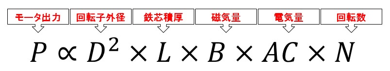
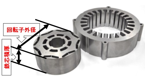
Fig.1-1 Motor output formula
2. Iron loss is the sum of eddy current loss and hysteresis loss
Iron loss is the sum of eddy current loss and hysteresis loss.
The eddy current loss can be reduced by thinning the electromagnetic steel sheet. For example, steel material 35H440 has a thickness of 0.35 mm. If technologies that can be further thinned advance, eddy current loss can be reduced considerably (Fig.2-1). Furthermore, as the eddy current decreases, the demagnetizing field component in the electromagnetic steel sheet decreases, and as a result, the effect of increasing the magnetic flux density with a small magnetic field has been reported (Fig.2-2). This means that the coil current for exciting the magnetic field can be made small, and reduction of copper loss can be expected.
The hysteresis loss corresponds to the area of the hysteresis curve. However, a slight increase in hysteresis loss occurs. The problem of measures to reduce the remaining hysteresis loss becomes important (Fig.2-3).

Fig.2-1 Decrease in eddy current loss due to thinning of electromagnetic steel sheet
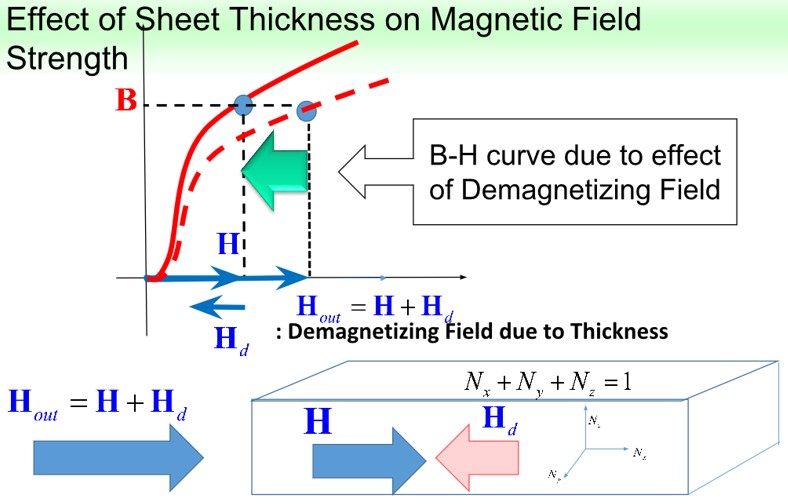
Fig.2-2 Reduction of magnetoresistance by thinning of electromagnetic steel plate
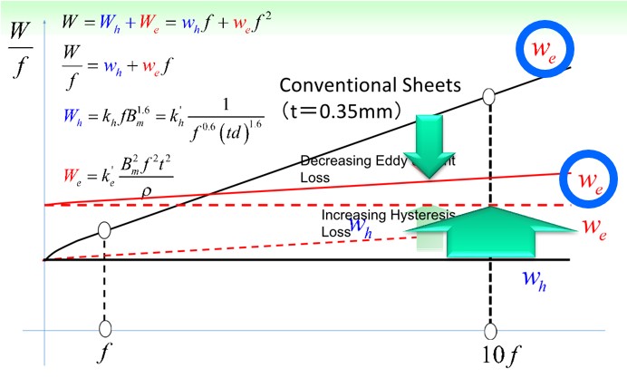
Fig.2-3 Hysteresis loss increases due to thinning of electromagnetic steel sheet
3. Vector magnetic properties of electromagnetic steel sheet
Measures to reduce iron loss of electromagnetic steel sheet, but conventionally it was the following method. Distribution of magnetic flux density is calculated by electromagnetic field analysis. Iron loss model (proportional to exponentiation of magnetic flux density) is used to estimate iron loss distribution and iron loss amount (Fig.3-1). Then design to lower core loss, you have to lower the magnetic flux density. In this way the traditional approach has been stalled.
Actually, the magnetic flux density and the magnetic field are constantly changing inside the electromagnetic steel plate used for the motor core. Alternating magnetic flux (magnetic flux density changes in one direction) and rotating magnetic flux (magnetic flux density rotates) occur depending on the location. Similarly, the magnetic field also changes, but when measured in detail, the direction of the magnetic flux density and the direction of the magnetic field are misaligned. For example, the magnetic field rotates before the rotating magnetic flux or it is delayed halfway. In this way, the relationship between the magnetic flux density and the magnetic field can not be accurately expressed unless consideration is given to the magnitude and direction (vector) (Fig. 3-2).
The magnetic field H and the magnetic flux density B were vector related when a technology capable of accurate measurement was made. As a result, since hysteresis loop can be drawn and its area is iron loss, we have learned that grasping this vector magnetic characteristic is very important.
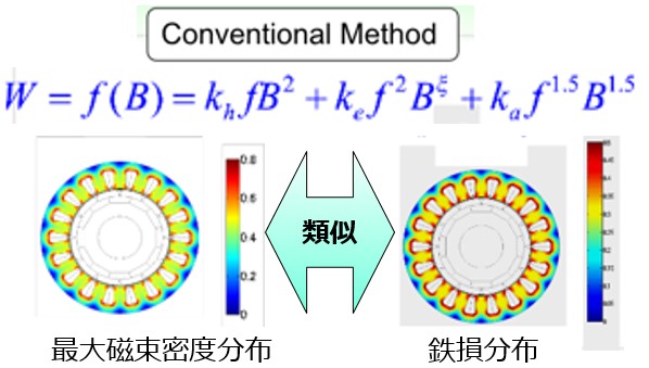
Fig.3-1 Similar distribution of magnetic flux density and iron loss in iron loss formula
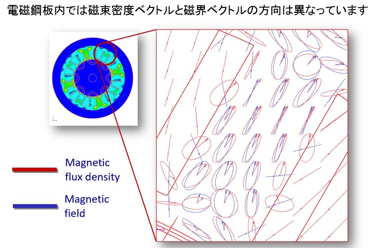
Fig.3-2 Lissajous waveform with magnetic field H and magnetic flux density B vector
4. Conventional measurements are scalar magnetic measurements
The current material measurement method is said to be scalar magnetic measurement. The Epstein tester and single plate magnetic tester measure excitation in one direction and measure the relationship between the magnetic flux density and the magnitude of the magnetic field in that direction. The result is a BH curve. Because it performs magnetic field analysis based on this information, it is scalar magnetic field analysis. Scalar magnetic field analysis (though it is considered as anisotropy) is performed by scalar magnetic measurement even if magnetic steel sheet is cut out in various directions and the magnetic characteristics are measured for each direction of the sample.
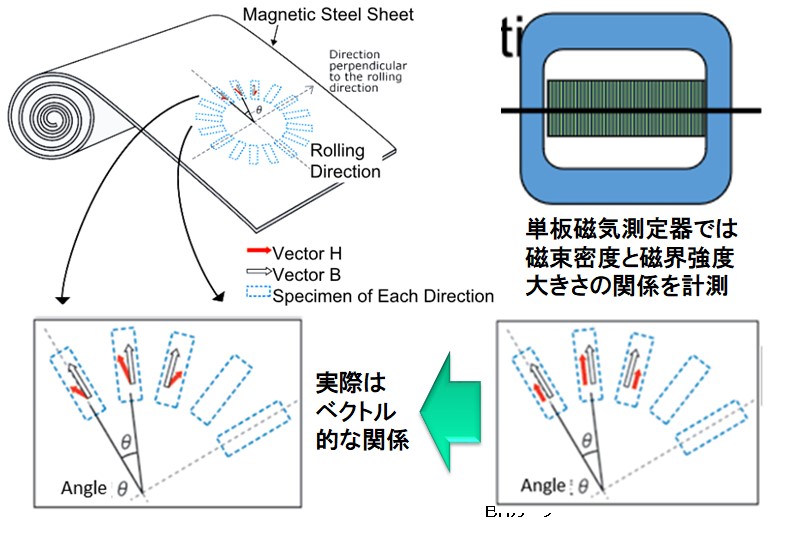
Fig.4-1 Current measurement is scalar magnetic measurement
5. Developed vector magnetometer
An alternating magnetic flux and rotating magnetic flux are generated in the electromagnetic steel plate of the motor and the transformer. Because it is excited by AC, it makes one revolution with one cycle of electrical angle. The alternating magnetic flux has a change that the magnetic flux density vector extends sinusoidally only with respect to a certain direction and then shrinks and then extends and shrinks in the opposite direction. However, also at this time, it can be observed that the trajectory of the magnetic field vector swells in a two-dimensional plane (Fig.5-1). This means that the magnetic field vector is oriented in a direction different from the magnetic flux density vector. It is a vector magnetic characteristic which can not be observed by scalar magnetic measurement.
A two-dimensional vector magnetometer has been developed that generates alternating magnetic flux and rotating magnetic flux and measures the magnetic field at that time (Fig 5-2). The excitation yokes are arranged in the rolling direction and the direction perpendicular to the rolling direction with respect to the specimen of the electromagnetic steel plate to generate the alternating magnetic flux and the rotating magnetic flux and measure the strength of the magnetic field. As a result, the magnetic property information of the electromagnetic steel sheet leaps from scalar to vector. Currently, Metron Technologies Inc. commercializes it as a vector BH tester (Fig.5-3). Accurate material characteristics can be obtained considering rolling direction of electromagnetic steel sheet. Vector magnetic characteristic analysis is to analyze iron loss using this material characteristic. For example, it is possible to calculate accurate hysteresis loss distribution which could not be obtained conventionally.
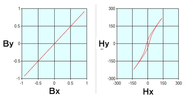
Fig.5-1 Rotating magnetic field for alternating magnetic flux (50 A 470, 1.3 Tesla)
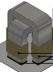
Fig.5-2 Two-dimensional vector magnetometer
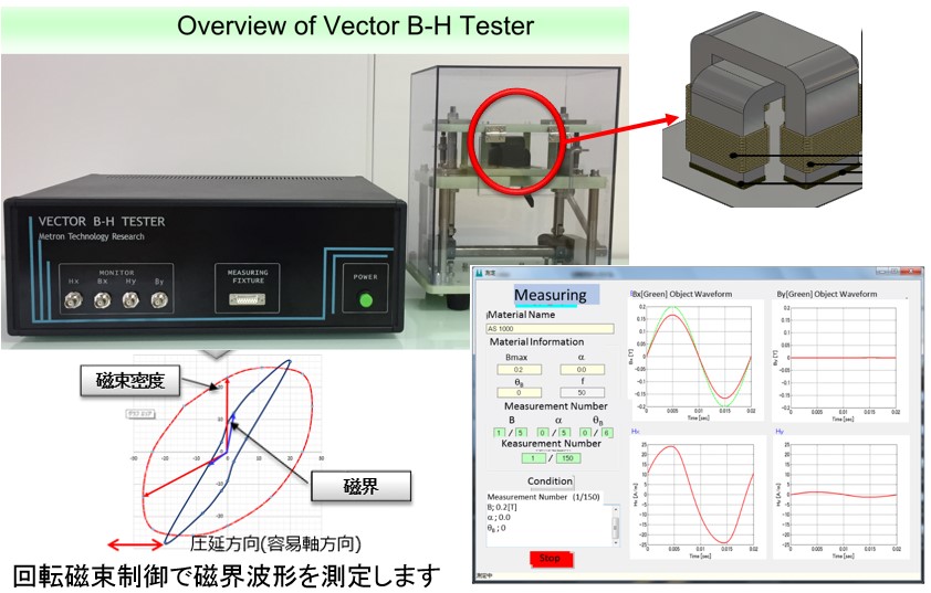
Fig.5-3 Vector BH tester (provided by Metron Giken)
6. Actual measurement result
It is the result actually measured by two-dimensional vector magnetometer (Fig 6-1). The rotating magnetic flux density vector (red mark) is controlled to rotate to a true circle with a size of 1.0 T. It is the rotation locus of the magnetic field intensity vector (blue mark) at that time. The rolling direction of the electromagnetic steel sheet is set in the X axis direction.
Even with non-oriented electrical steel sheet, anisotropy is seen in the direction perpendicular to the rolling direction. The rolling direction has a tendency of easy magnetization, and the magnetic field strength for obtaining magnetic flux density 1.0 T is small. Since the magnetic flux density of 1.0 T can be achieved with a large magnetic field strength in the perpendicular direction, the Lissajous waveform of the magnetic field is vertically long. This tendency is more pronounced in directional electromagnetic steel sheets and bidirectional magnetic steel sheets. And the vector direction is different. It became possible to measure like this.
Then, in order to utilize these as magnetic characteristic data, we first create a database. Then, utilizing the database like the BH curve of the scalar magnetic field analysis is vector magnetic characteristics analysis technology.
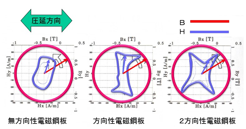
Fig.6-1 Difference in vector magnetic characteristics depending on the type of electromagnetic steel sheet
7. Making database as magnetic characteristics
By using vector magnetometer, alternating magnetic flux and rotating magnetic flux are generated with respect to the specimen of electromagnetic steel plate, a number of distorted magnetic field intensity waveforms corresponding to it are measured and registered as a vector magnetic property database. Data is organized by three parameters (Fig.7-1).
In order to express from a true circle to an ellipse and an alternating magnetic flux having no area, the ratio of the magnetic flux density Bmax of the major axis of the ellipse to the Bmin of the minor axis is the axial ratio α. α = 1 is a perfect circle and α = 0 is an alternating magnetic flux. Next, the direction of the ellipse of the rotating magnetic flux, the angle of inclination θ B is how many times it is inclined counterclockwise with respect to the rolling direction. Finally, let's set the magnitude of the maximum magnetic flux density Bmax itself as a parameter that changes from 0.0 Tesla to 1.6 Tesla. For example, the distorted magnetic field strength waveform for one period of electrical angle is stored under the condition of 3230 kinds of axial ratio 10 points, inclination angle 19 points, maximum magnetic flux density 17 points. Actually, the distorted magnetic field intensity waveform is represented by a Fourier series, and the maximum degree is 51st order and so on. The capacity of this database is around 100 Mb.
This magnetic property data is very valuable, and various information can be seen from here (Fig. 7-2). For example, the iron loss characteristics with respect to the inclination angle and the scalar BH curve are included in the information in this. On the website, we are planning to develop its characteristic chart as "visualization of magnetic properties". Then, vector magnetic characteristic analysis is carried out referring to this database.
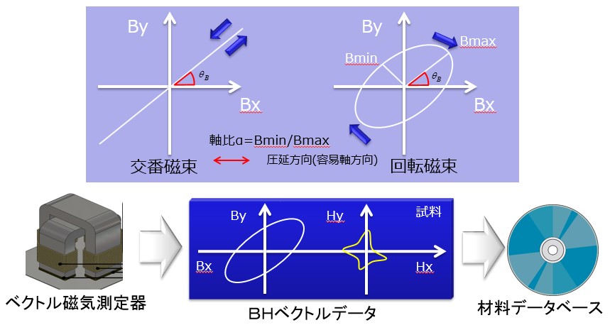
Fig.7-1 Two-dimensional vector magnetic property database
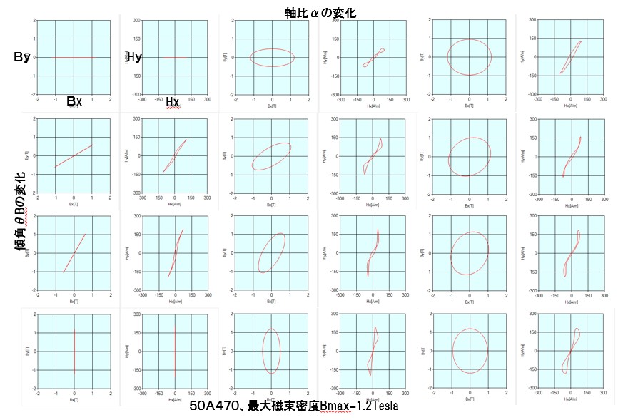
Fig.7-2 Lissajous waveform of magnetic flux density and magnetic field strength at parameter change
8. What is the E & S model?
The E & S model is a numerical model that expresses the relationship between the magnetic flux density vector B and the magnetic field strength vector H obtained by the two-dimensional vector magnetic characteristics. Furthermore, I think that it is an algorithm applied to the magnetic property analysis using the finite element method.
The relational expression between B and H of E & S model is shown (Fig.8-1). This model calculates the sum of the product of the magnetic flux density waveform multiplied by the magnetoresistive coefficient (νxr, νyr) and the product of the integral waveform of the magnetic flux density waveform multiplied by the magnetic hysteresis coefficient (νxi, νyi) It is a method of obtaining. Due to the magnetic hysteresis coefficient, the magnetic field strength is designed to have a value even under conditions such that Bx and By are zero at the same time. The magnetoresistance coefficient and magnetic hysteresis coefficient are calculated from the magnetic flux density and magnetic field intensity waveform of each condition (Bmax, θB, α) stored in the vector magnetic property database. τ is a dividing point with one period of electrical angle, and the magnetoresistive coefficient etc is also the waveform of one period of electrical angle (Fig.8-2). In the actual calculation, the Fourier coefficients of the magnetoresistive coefficient and the magnetic hysteresis coefficient can be determined by developing and calculating the magnetic flux density waveform and the magnetic field strength waveform to Fourier series, and finally returning to the time axis waveform. The calculation time of this calculation is not required.
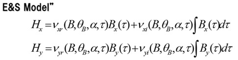
Fig.8-1 Relationship between B and H of the E & S model
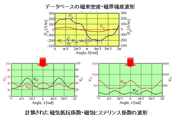
Fig.8-2 Waveforms of magnetoresistive coefficient and magnetic hysteresis coefficient
9. E & S model flowchart
The calculation of the E & S model is based on one rotation flux (electrical angle) cycle. The flowchart is shown (Fig.9-1). First, we perform magnetic field analysis for one cycle under initial conditions. From the waveform result of magnetic flux density for each element, take out the fundamental waveform Fourier series. Calculate the maximum magnetic flux density Bmax (major axis value), minimum magnetic flux density Bmin (minor axis value), inclination angle θ B (rolling direction and angle of Bmax) and axial ratio α (Bmax / Bmin) from this basic waveform. Based on this information, find the corresponding rotating flux from the database and extract the magnetic field waveform at that time. Calculate the magnetic resistance coefficient and magnetic hysteresis coefficient waveform for one period from magnetic flux density and magnetic field, and use this to perform magnetic field analysis for the second cycle. We will do this until convergence (change of waveform becomes sufficiently small). The result of convergence is a result that is in line with the material characteristics actually measured by each element. Finally, find the hysteresis curve from the magnetic flux density / magnetic field waveform and calculate the iron loss. Vector magnetic characterization The overall flow of analysis is shown (Fig.9-2).
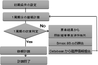
Fig.9-1 E & S model flowchart
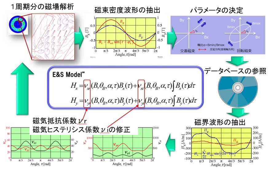
Fig.9-2 Flow of overall vector magnetic characteristics analysis
10. Analysis considering rolling direction
Electric steel sheets are easy to pass through the magnetic flux in the rolling direction even in non-directional (50 A 470 in the example), and there is a tendency for magnetic steel sheets to be hard to pass in the direction perpendicular thereto. It is reproduced by vector magnetic character analysis (Fig.10-1).
It is a model that excites by winding a coil around an electromagnetic steel plate cut into a ring shape. The rolling direction is the X axis (horizontal direction). Vector magnetic character analysis result Contour diagram is shown. The magnetic flux density distribution is almost uniform in the circumferential direction, the inner diameter side with a short magnetic path length has a large value. On the other hand, the magnetic field distribution shows large values in the left and right parts. This is because the magnetic flux tends to flow through the upper and lower portions where the magnetic flux density vector faces the X axis and is aligned in the rolling direction and the resultant magnetic flux density is obtained even with a small magnetic field. On the contrary, in the right and left parts, the flow of magnetic flux and the rolling direction are perpendicular, the magnetic flux hardly passes, and the resultant magnetic flux density is achieved with a large magnetic field. The iron loss distribution obtained from the magnetic flux density and the magnetic field also has large values in the left and right parts under the influence of the rolling direction.
The result which can not be obtained by the conventional scalar magnetic characteristic analysis is a basic problem which can be calculated by vector magnetic characteristics.
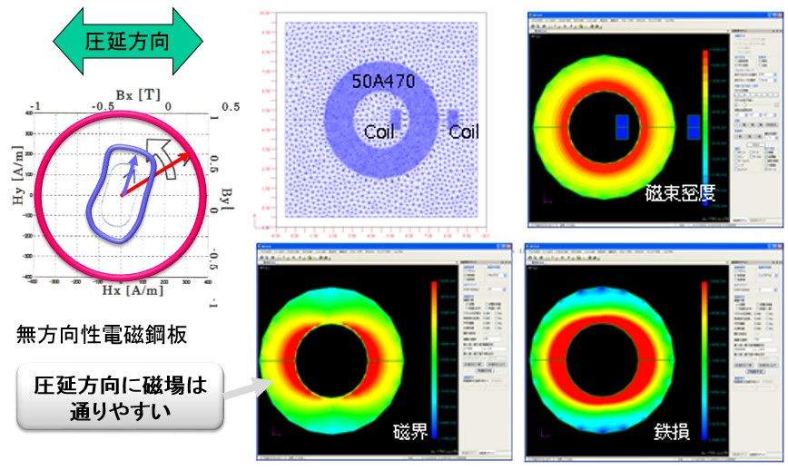
Fig.10-1 Influence of rolling direction
11. Comparison with conventional analysis method
In the conventional iron loss calculation method for scalar magnetic characteristic analysis, the iron loss distribution was obtained by post-processing using the iron loss formula from the result of magnetic flux density. Therefore, the magnetic flux density distribution and iron loss distribution are similar distribution. On the other hand, in vector magnetic characteristics analysis, the iron loss distribution differs from the magnetic flux density distribution. This is because it takes into consideration the influence of the magnetic properties in the rolling direction (Fig. 11-1). Also in iron loss analysis considering hysteresis, accurate iron loss distribution can not be obtained if hysteresis material characteristics are obtained from scalar measurements. Vector magnetic characteristics analysis has characteristics that magnetic field distribution can be accurately calculated. This is because we refer to measured data of magnetic flux density and magnetic field strength of vector magnetic property database (Fig.11-2). Furthermore, since a hysteresis loop can be drawn from the magnetic flux density waveform and the magnetic field intensity waveform and its area is iron loss, iron loss value and iron loss distribution can be calculated accurately (Fig.11-3).
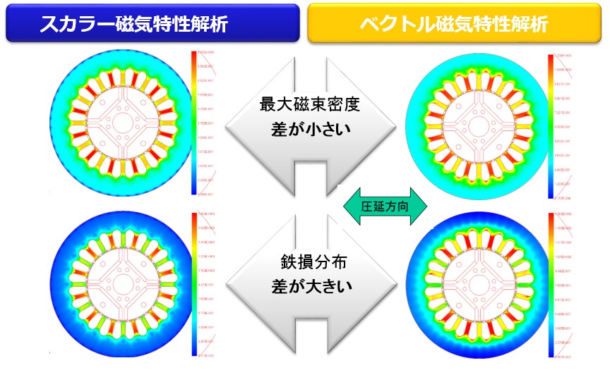
Fig.11-1 Comparison with conventional scalar analysis method
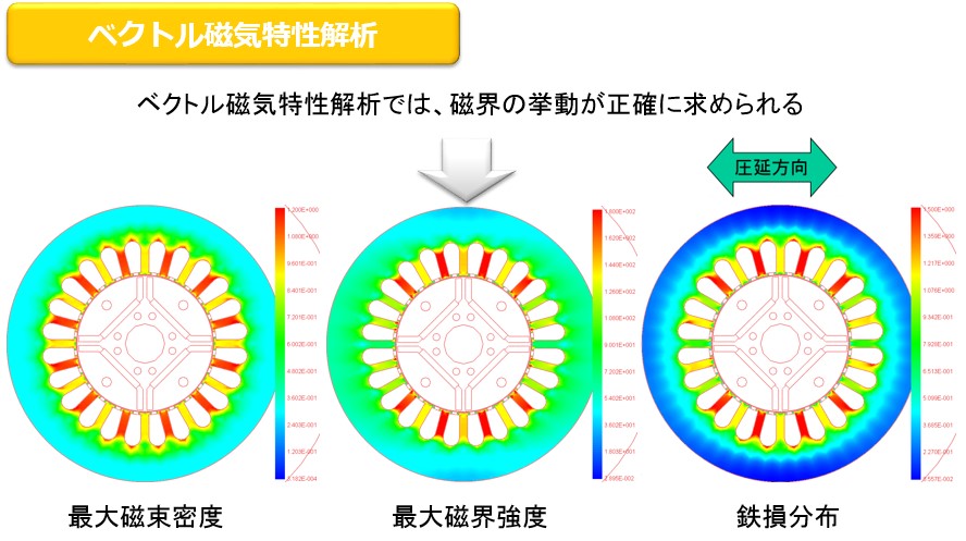
Fig.11-2 Accurate magnetic field distribution
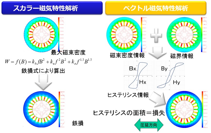
Fig.11-3 Iron loss distribution with good accuracy
12. Measures to reduce iron loss
If you know the accurate iron loss distribution by vector magnetic character analysis, we will take measures against places where many iron losses are occurring. For example, we will repeat the case study analysis by changing the shape (shape and radius) of the stator (Fig.12-1). In the split core type (Fig.10), the core loss is reduced by dividing the stator core so that the rolling direction and the magnetic flux direction agree (Fig.12-2).
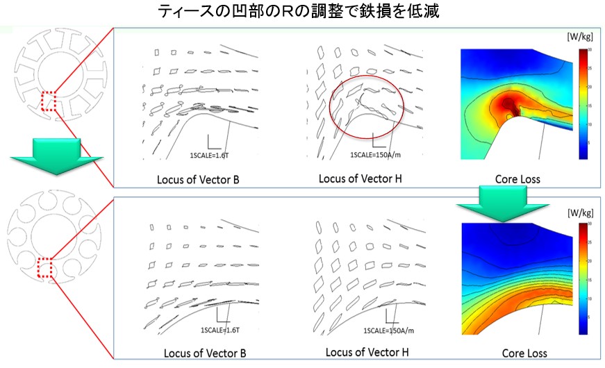
Fig.12-1 Example of measures to reduce iron loss
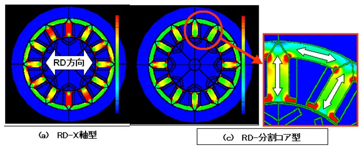
Fig.12-2 Measures to reduce iron loss of stator by split core type
13. Parameters that serve as a clue to iron loss reduction countermeasures
The parameters mentioned here show the relationship between these parameters and core loss at each θBH of the A and B vectors and the H vector used in the vector magnetic characteristic measurement as well as the axis ratio α and the inclination angle θ B (Fig.13- 1). If we can grasp such a tendency, we can design as a design devised to change various parameters in the direction of iron loss reduction. It also has a function to contour display the distribution of various parameters (Fig.13-2).
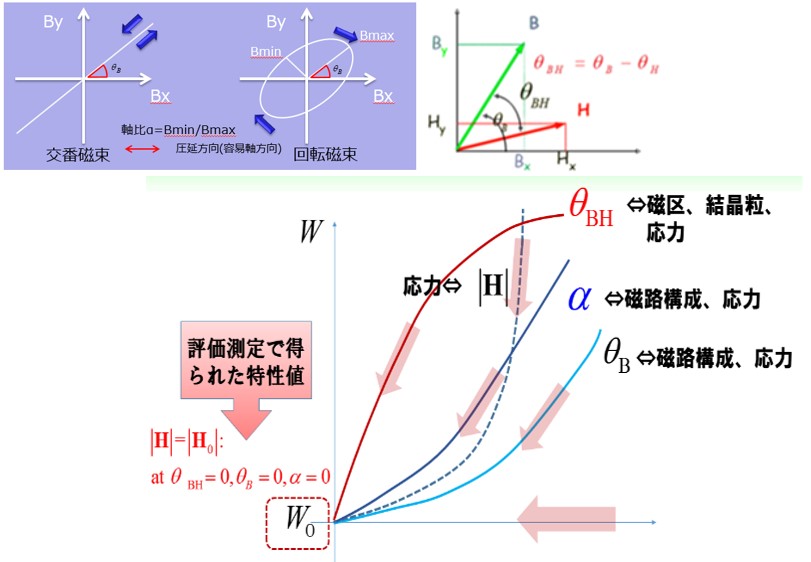
Fig.13-1 Iron loss reduction measures devised from parameters
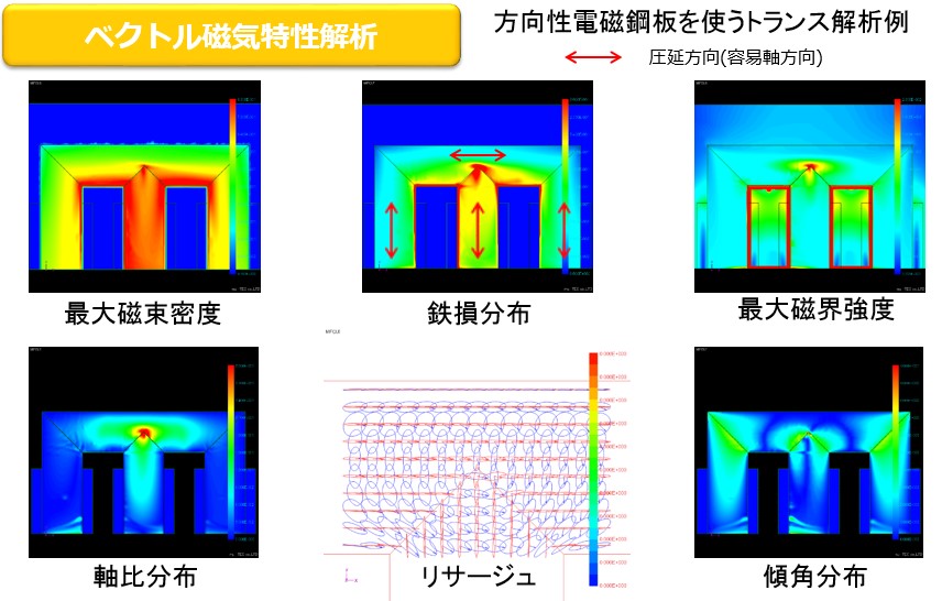
Fig.13-2 Example of parameter contour display
14. Development into dynamic E & S model
We have discussed vector magnetic characteristics analysis so far, but this algorithm consists of a static E & S model algorithm. Measured by the vector magnetic property measuring device is a distorted magnetic field strength vector waveform generated when the magnetic flux density vector is excited by a sinusoidal wave. In addition, since the measurement is 50 Hz excitation, eddy current due to 50 Hz is taken into consideration. Using this magnetic flux density B vector and magnetic field intensity H vector, hysteresis curves of x component and Y component can be drawn. Since this hysteresis curve also includes the effect of eddy current of 50 Hz, the area integral of the hysteresis curve is 50 Hz iron loss (hysteresis loss + eddy current loss).
The challenge is the iron loss at frequencies other than 50 Hz (Fig.14-1). On actual machines, use at higher frequencies is considered. Another problem is correspondence to the distorted magnetic flux density waveform. Since it is a static E & S model that the magnetic flux density is excited by a sinusoidal wave, we extracted the fundamental wave component of the distorted magnetic flux density waveform and referenced the database. The dynamic E & S model addresses these two challenges.
In the dynamic E & S model, the magnetic field strength due to the eddy current of the operating frequency is calculated and corrected using the classic eddy current model (modeling the eddy current in the thin plate). For the distorted magnetic flux density, decompose it into harmonic components, calculate the influence of eddy currents in that frequency component, and correct it. In this way you will be able to simulate more realistic vector magnetic properties relationships.
The dynamic E & S model will be incorporated as a grade-up of μ-E & S soon.
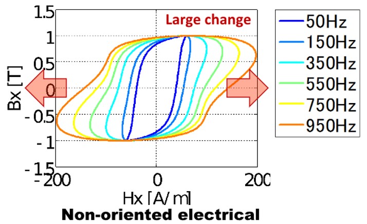
Fig.14-1 Frequency dependence of hysteresis curve
15. Consider the influence of stress
A lot of presentations on the influence of stress have already been made in the study of vector magnetic property technology centered on Professor Enokizono. For details, please refer to the homepage of "Vector Magnetic Property Technology Institute". Implementing the function to μ-E & S is still a story before.
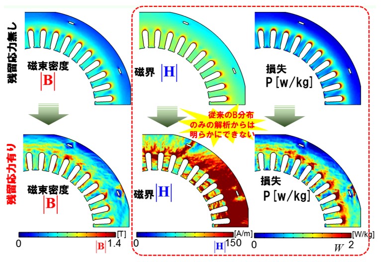
Fig.15-1 Iron loss analysis considering residual stress
16. Function table of μ-E & S
| Analysis type | Two-dimensional transient magnetic field analysis (FEM) |
|---|---|
| algorithm | E & S model |
| excitation | Voltage source, current source, permanent magnet |
| Material Database | 4 directional and non-oriented electrical steel sheets |
| Target motor | Synchronous motor (Inductive motor is under development) |
| Model input | FemapNEU file (Separately own company mesher - included) |
| Output (numerical value, figure) | Hysteresis loop, iron loss, current waveform, maximum magnetic flux density, maximum magnetic field strength, inclination angle, axial ratio, torque |
| GUI | Easy to use interface of wizard system |
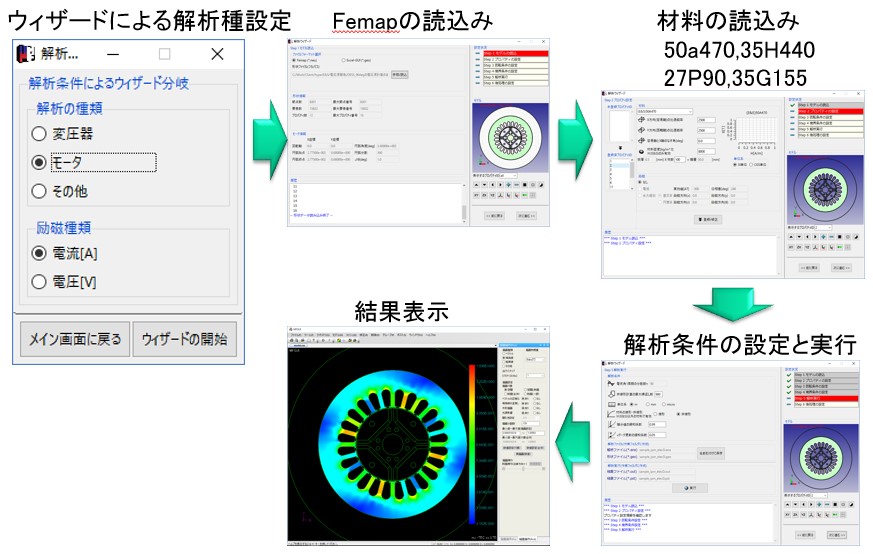
Fig.16-1 Interface of μ-E & S