

Analysis example collection (1) Ring model voltage source
table of contents
1. Analysis model and purpose
The analysis model diagram is shown in Fig. The analysis model assumes a model in which a non-oriented electrical steel sheet (50 A 470) is launched into a ring shape. Input the voltage to the exciting coil and excited so that the maximum magnetic flux density becomes about 1.6 T. The rolling direction of the electromagnetic steel sheet is the X direction. This model is an analysis model for confirming that there is magnetic anisotropy in the rolling direction even if the electromagnetic steel sheet is non-oriented. In addition, although every part becomes an alternating magnetic flux, since the rotating magnetic field is seen in the measurement of vector magnetic characteristics, we also confirm that it can be calculated.
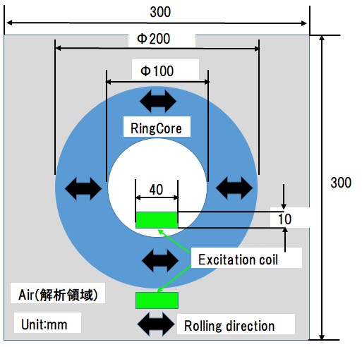
Fig.1.1.1 Model diagram
2. Analysis conditions and calculation time
The mesh model used for analysis is shown in Fig.1.2.1 and the analysis condition is shown in Fig.1.2.2. The voltage condition is set so that the maximum magnetic flux density is about 1.6 T (In the case of calculation by current input, the total current amount of the coil becomes approximately 35 (Aturn)). The computation time was about 8 min (Intel Core i 5, 28 GHz machine), the nonlinear iteration converged at 216 times.
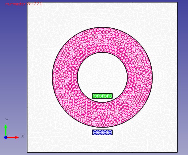
Fig.1.2.1 Mesh model
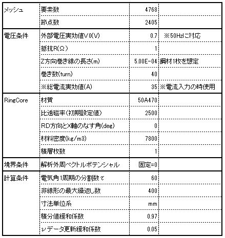
Fig.1.2.2 Analysis condition
3. Magnetic field distribution, iron loss distribution result
Maximum magnetic flux density distribution, maximum magnetic field intensity distribution, iron loss distribution are shown in Fig.1.3.1, Fig.1.3.2 and Fig.1.3.3. In the magnetic flux density distribution, the magnetic flux density is maximized in the upper and lower regions where the rolling direction and the magnetic flux density vector are parallel (inclination angle θ B = 0), and the magnetic flux density is uniformed to the left and right regions. This is the upper and lower region where the magnetoresistance in the rolling direction is small and the magnetic flux density concentrates on the inner diameter side with the shorter magnetic path length. Conversely, the magnetic field intensity distribution tends to have a large magnetic resistance in the left and right regions where the magnetic flux density vector is perpendicular to the rolling direction = the magnetic field strength is large. In the iron loss distribution, iron loss tends to be large in the upper and lower regions where the magnetic flux density is large, but also in the left and right regions as compared with the magnetic flux density distribution. This is because the iron loss is a scalar product of the magnetic flux density and the magnetic field strength, It is influenced by the area. In this way, the iron loss distribution showed the same tendency as the magnetic flux density distribution in the conventional calculation method, but in the vector magnetic characteristic analysis, it is shown that the iron loss distribution can be calculated considering the accurate magnetic field strength and its influence There.
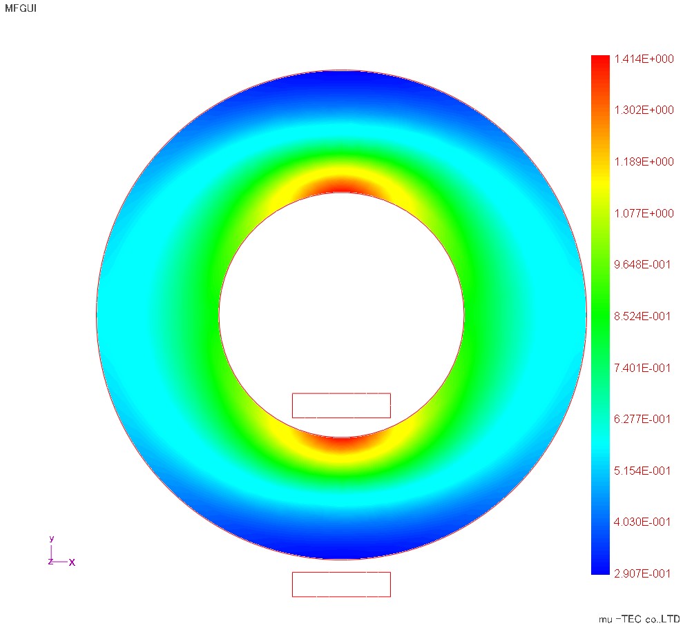
Fig.1.3.1 Maximum magnetic flux density distribution (indicated by maximum 1.41 T)
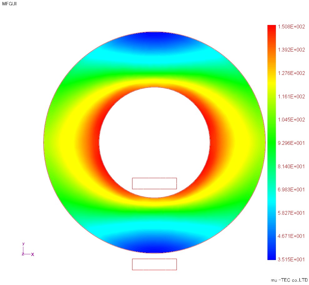
Fig.1.3.2 Maximum magnetic field strength distribution (indicated at maximum 150 A / m)
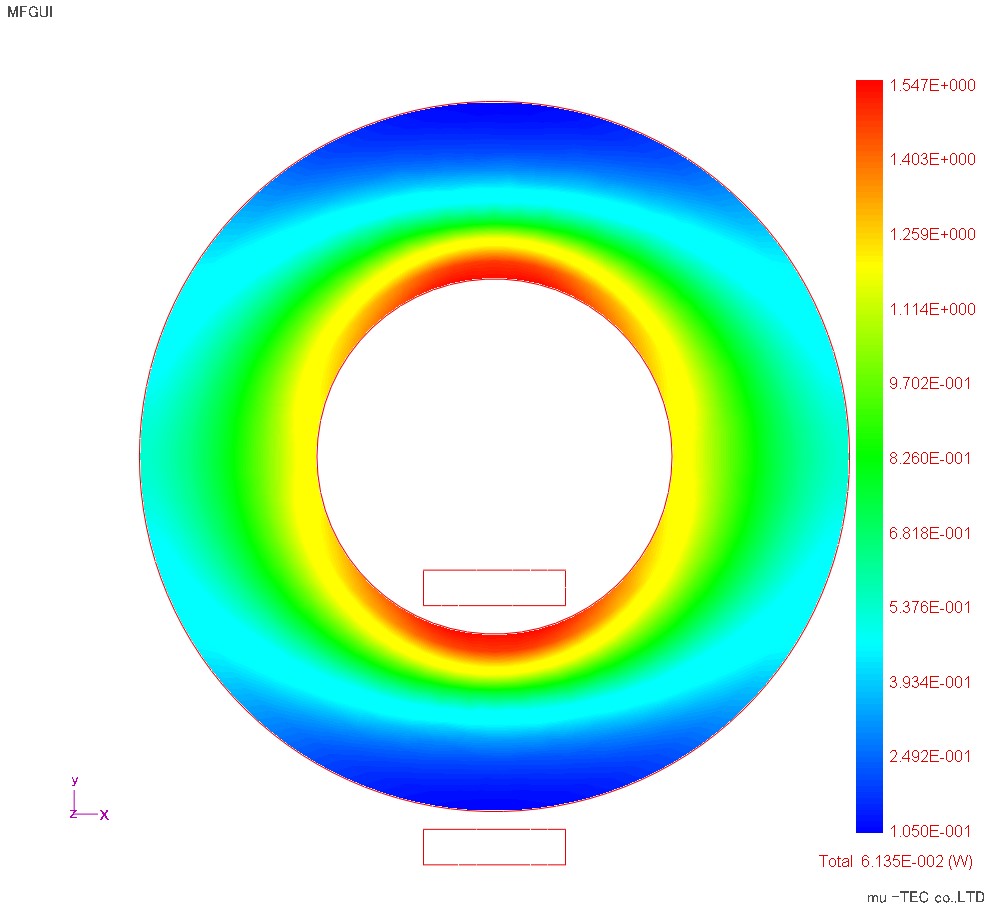
Fig.1.3.3 Iron loss distribution (indicated at maximum 1.5 W / kg) (The total iron loss value of one laminated layer considered in the model is 0.135 e -2 (W))
4. Alternating magnetic flux and rotating field result
Fig.1.4.1 is a diagram in which the Lissajous waveform of the magnetic flux density vector (red) and the magnetic field intensity vector (blue) is normalized (the waveforms are displayed with the same magnitude). The Lissajous waveform of the red magnetic flux density vector is an alternating magnetic flux (not a rotating magnetic flux), and its direction changes cleanly concentrically. In addition, Fig.1.4.2 is a display that is not normalized, and it can be confirmed that the Lissajous waveform becomes smaller as going to the outer diameter side. Furthermore, Fig.1.4.3 shows an enlarged view of the Lissajous waveform at the circle in Fig.1.4.1 (a position at an angle of 45 degrees). In this figure, the magnetic flux density vector (violet) is an alternating magnetic flux in the direction of 135 degrees, but the magnetic field intensity vector (green) is a rotating magnetic field with the slope in the direction of 120 degrees. This result is also the calculation result obtained from the vector magnetic characteristic measurement result.
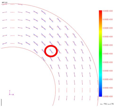
Fig.1.4.1 Lissajous waveform (Normalization)
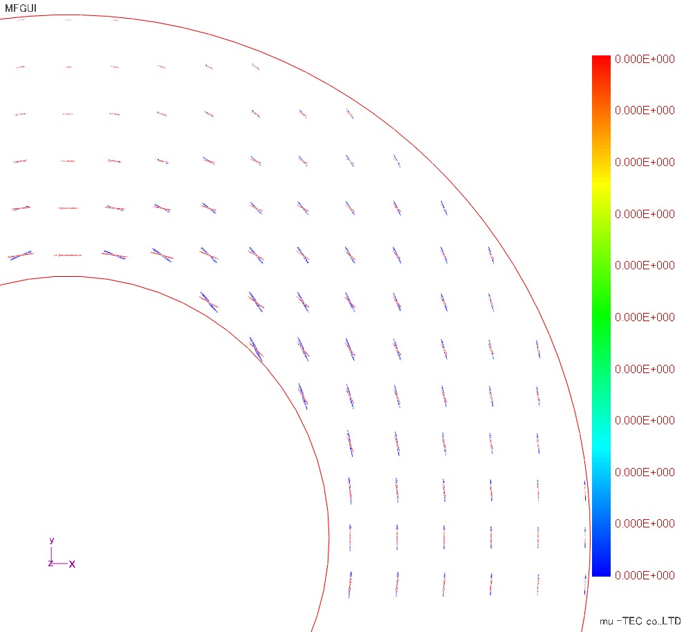
Fig.1.4.2 Lissajous waveform (no normalization)
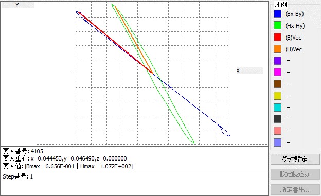
Fig.1.4.3 Enlarged display of Lissajous waveform (purple: magnetic flux density, green: magnetic field strength)
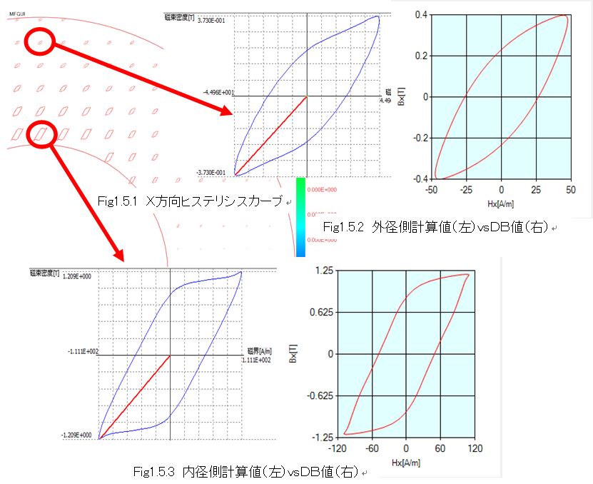
5. Result of comparison with measured value of hysteresis curve
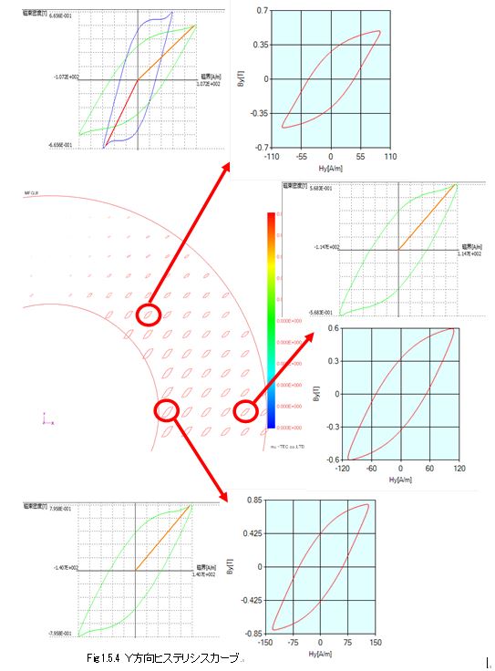
Fig. 1.5.1 shows the distribution of X direction hysteresis curves (curves based on Hx and Bx). The circle is the location in the 0 o'clock direction of the ring specimen where the alternating flux is only in the X direction. The hysteresis on the outer diameter side of the ring sample with a low magnetic flux density is shown in Fig. The maximum value of the magnetic flux density of 0.37 T and the maximum magnetic field strength of 45 A / m, and the corresponding DB (in the database) values are shown on the right, but they agree well. The DB value referred to is the waveform with the maximum magnetic flux density Bmax = 0.4 T, the inclination angle θ B from the rolling direction of the alternating magnetic flux, 0, and the axial ratio α = 0 representing the alternating magnetic flux. Since the DB value is the measured value itself in this condition, it can be considered that the calculated result agrees well with the measured value. Since the E & S algorithm of the vector magnetic characterization analysis performs the magnetic field analysis of the finite element method with the database of the measured waveform as the material characteristic, the calculation result coincides with the waveform of the database and it is said that it coincides with the measured value accurately I can say things. Similarly, the hysteresis on the inside diameter side of the ring specimen with a large magnetic flux density is shown in Fig. 1.5.3, but the calculation result and the DB value are in good agreement with each other. For the Y direction hysteresis curve in Fig. 1.5.4, the calculation result of each place and the DB value are compared and the consistency is confirmed.
6. Current waveform result
Although the excitation method is given by voltage source and current source, current waveform is obtained as a result because it is voltage source system this time (Fig 1.6.1). Since the maximum current value is about 1 A and the condition of 40 turns, the total current amount is about 40 Aturn. In the waveform, it is compared with the COS wave, but the obtained current value is distorted. For example, as the magnetic flux density increases further, saturation occurs and the magnetic resistance increases, so that the waveform peak is close to a sharp triangular wave. In this way, nonlinearity of the magnetic characteristics can be taken into consideration, so calculation by the voltage source method is desirable.
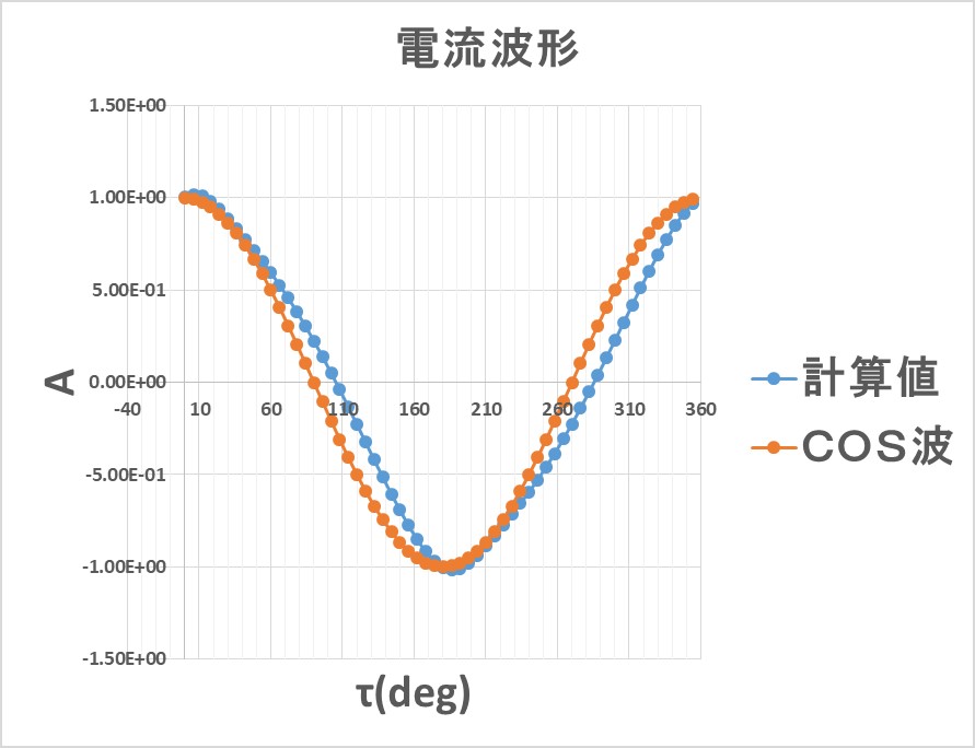
Fig.1.6.1 Current waveform
7. Interface setting screen
Here, we introduce the procedure of μ-E & S in order of interface screen.

Fig.1.7.1 Activation of μ-E & S
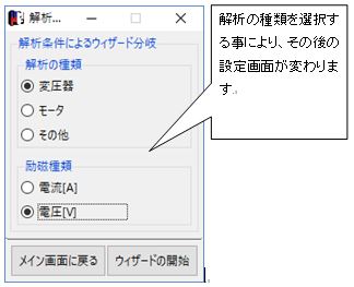
Fig.1.7.2 Selection of analysis type by analysis wizard
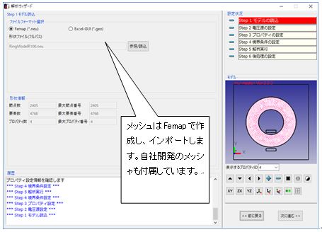
Fig.1.7.3 Import of ring model created by Femap
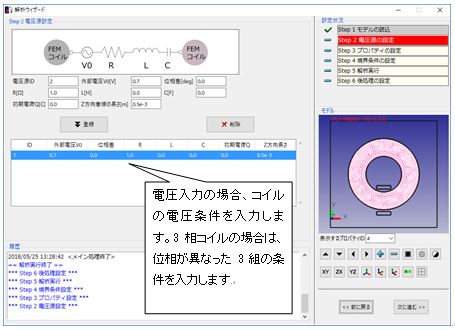
Fig.1.7.4 Setting of voltage condition
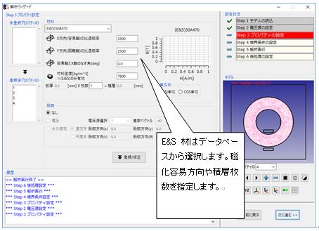
Fig.1.7.5 Material setting
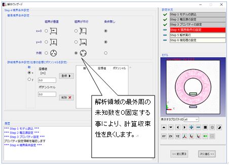
Fig.1.7.6 Setting boundary condition
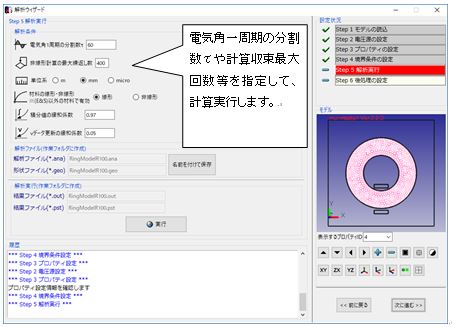
Fig.1.7.7 Analysis condition setting and calculation execution such as convergence count
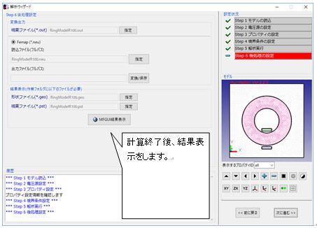
Fig.1.7.8 Preparation of result display
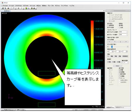
Fig.1.7.9 Result display
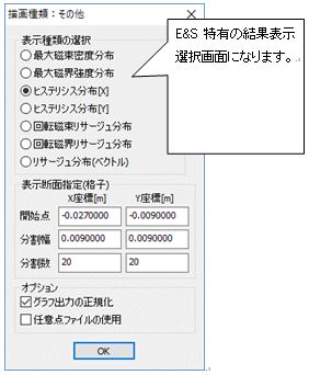
Fig.1.7.10 Setting hysteresis and Lissajous waveform