


Analysis example collection (2) Ring model voltage source (difference in steel material)
table of contents
1. Analysis model and purpose
Using the analysis model of the ring specimen used in Analysis Case 1 (Fig 2.1.1, Fig 2.1.2), confirm the change due to the difference in steel material. The steel material is a non-oriented electrical steel sheet with 50 A 470 and 35 H 440. Input the voltage to the exciting coil and excited so that the maximum magnetic flux density becomes about 1.6 T. The rolling direction of the electromagnetic steel sheet is the X direction. Since the plate thickness of the steel material is different, the laminate number was changed to make the product thickness same, and the voltage condition and so forth of the coil were the same.
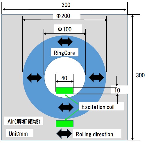
Fig.2.1.1 Model diagram
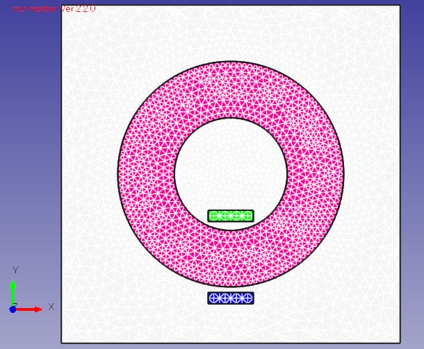
Fig.2.1.2 Mesh model
2. Analysis conditions and calculation time
The analysis conditions are shown in Fig.2.2.1. Since the thickness of the steel material is different, the number of laminated sheets was changed and the product thickness was made the same, therefore the same voltage condition was set. Computation time converged at about 11 to 14 min (IntelCorei 5, 28 GHz machine) and nonlinear iteration at 300 to 400 times.
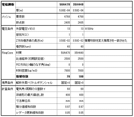
Fig.2.2.1 Analysis condition
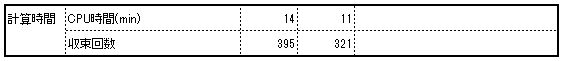
Fig.2.2.2 Calculation time and number of convergence
3. Magnetic field distribution, iron loss distribution result
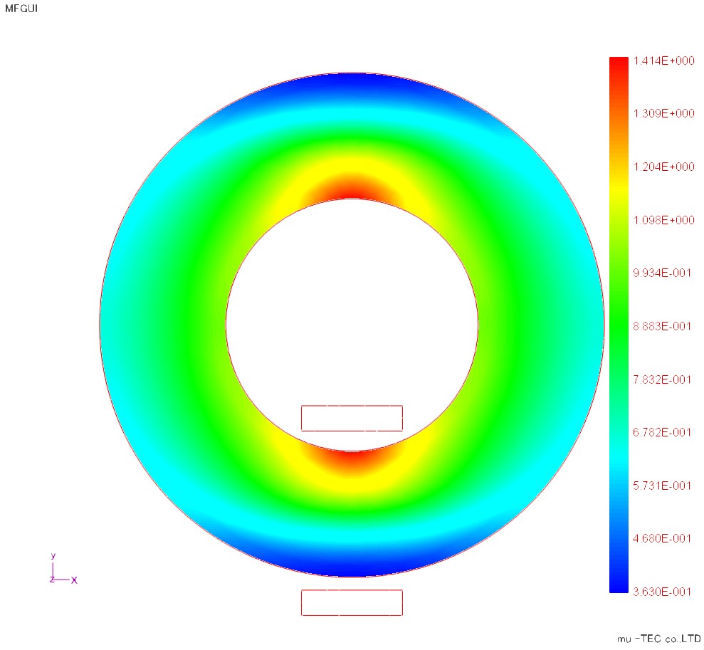
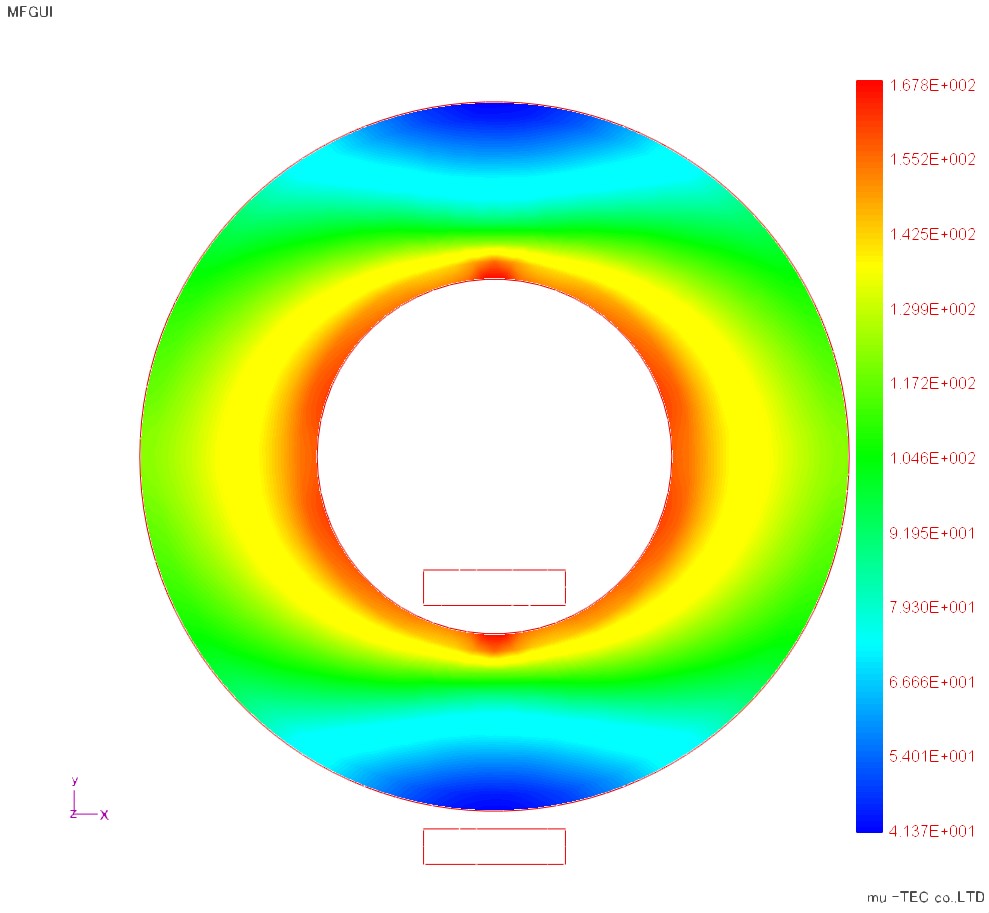
Maximum magnetic flux density distribution, maximum magnetic field strength distribution, iron loss distribution are shown in Fig 2.3.1, Fig 2.3.2, Fig 2.3.3. The magnetic flux density is larger at 35 H 440. The magnetic field intensity is smaller for 35H440. The iron loss distribution was almost the same distribution and size for both, and the total iron loss amount increased by about 3% by 50 A 470.
 |
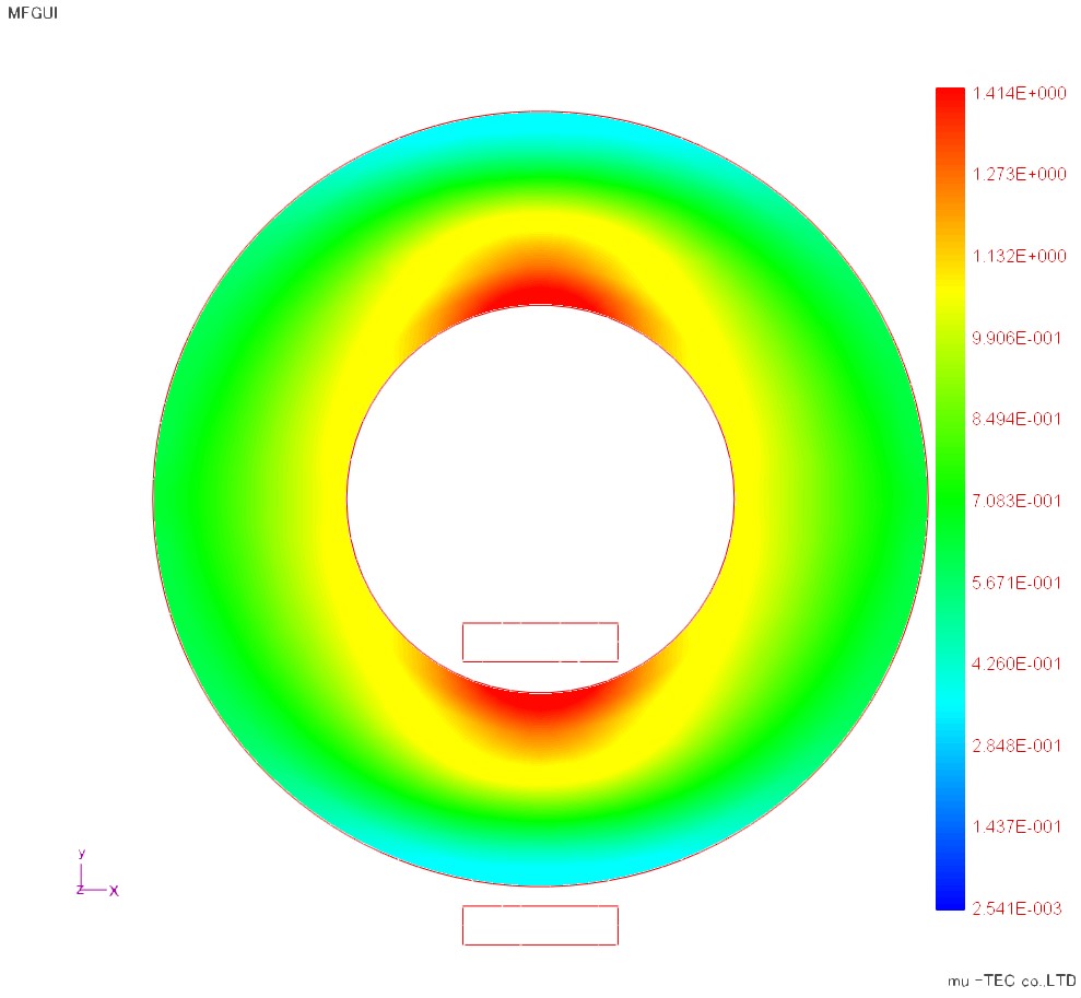 |
Fig.2.3.1 Maximum magnetic flux density distribution (indicated by maximum 1.41 T) Left: 50 H 470 Right: 35 H 440 |
|
 |
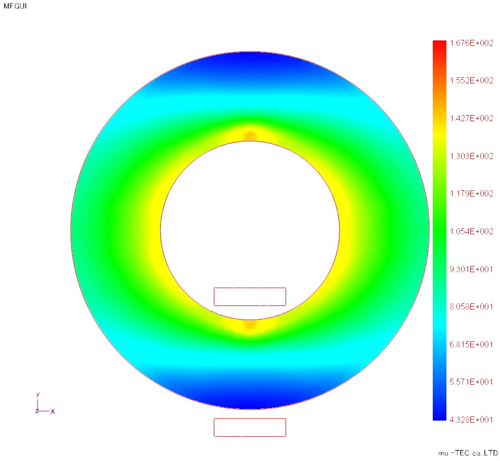 |
Maximum magnetic field intensity distribution (indicated by maximum 167 A / m) Left: 50 H 470 Right: 35 H 440 |
|
 |
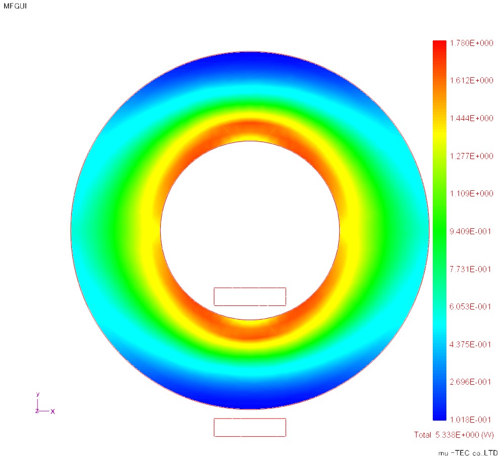 |
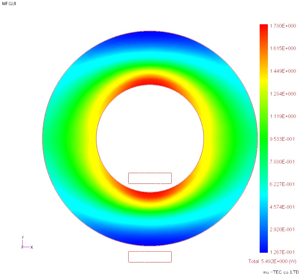
Fig.2.3.3 Iron loss distribution (indicated by maximum 1.7 W / kg) Total iron loss value is left: 50 A 470 5.492 (W) Right: 35 H 440 5.338 (W) |
|
4. X direction hysteresis curve result
Fig 2.4.1 shows 50 A 470 on the left side and 35 H 440 on the right side. The upper row shows the distribution of the X direction hysteresis loop (with normalization), the enlarged view of the blue circle in it is the middle stage, and the enlarged view of the red circle is the lower stage. The DB curve is also shown in the lower right corner.
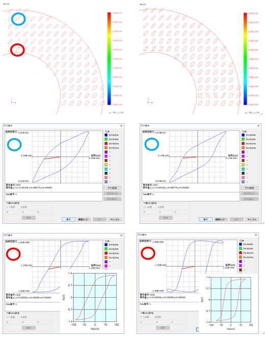
Fig.2.4.1 X direction hysteresis curve
5. Y direction hysteresis curve result
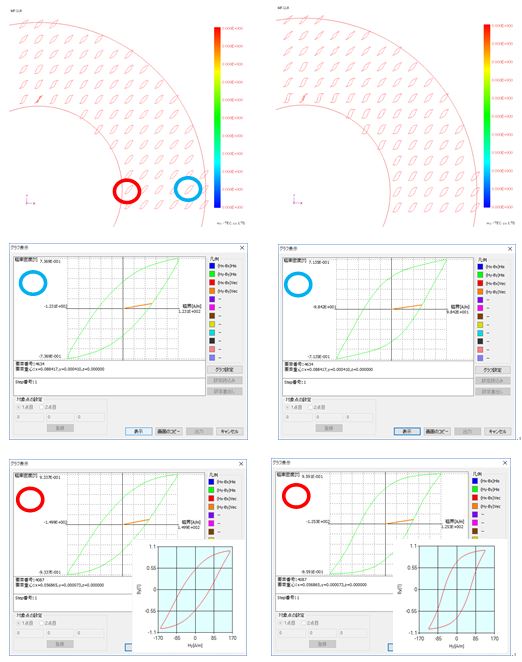
Fig.2.5.1 Y direction hysteresis curve
6. Current waveform result
Compare current waveforms. Looking at the DB hiss curve shown in the previous chapter 2.5.1, the 35 H 440 has a higher degree of rise than 50 A 470, which indicates that it is a material with a slightly higher permeability. As a result, as shown in Fig. 2.3.1 in the previous chapter, the magnetic flux density is increased even under the same excitation condition. In the comparison of the current waveforms, it is considered that the induced voltage increases with 35 H 440 when the magnetic flux density is larger, and the peak value of the current waveform has decreased. Furthermore, under the influence of magnetic saturation, the current waveform is sharper than 50 A 470.
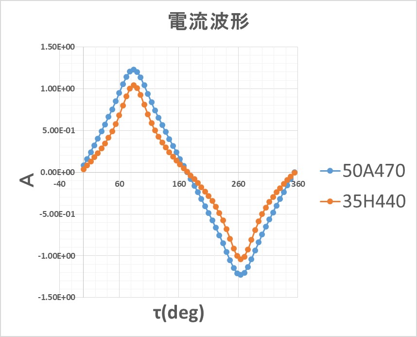
Fig.2.6.1 Current waveform