


Analysis example collection (3) Trans model (difference in directional material)
table of contents
1. Analysis model and purpose
Fig.3.1.1 shows a transformer model using directional materials. The transformer is a model combining three-phase three-leg transformer and directional material. Since the alternating magnetic flux is the basis in the transformer, the directional material is used, but the rotating magnetic flux is generated in the vicinity of the junction. Therefore, what kind of rotating magnetic flux is generated by analysis is confirmed. We also compare the directional electromagnetic steel sheets 27 P 90 and 35 G 155. Input the voltage to the exciting coil and excited so that the maximum magnetic flux density becomes about 1.0 T. Since the plate thickness of the steel material is different, the laminate number was changed to make the product thickness same, and the voltage condition and so forth of the coil were the same.
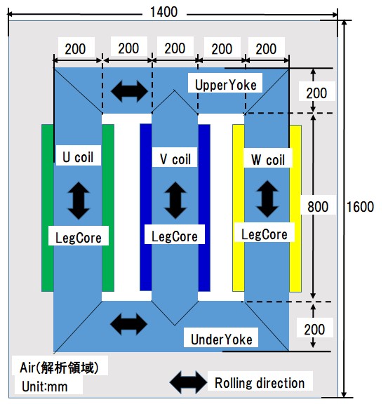
Fig.3.1.1 Model diagram
2. Analysis conditions and calculation time
The analysis conditions are shown in Fig.3.2.1. Since the thickness of the steel material is different, the number of laminated sheets was changed and the product thickness was made the same, therefore the same voltage condition was set. Computation time was about 39 min (IntelCorei 5, 28 GHz machine), nonlinear iteration converged at 360 times. The mesh diagram is shown in Fig. 3.2.3, and the Lissajous waveform evaluation point is shown in Fig. 3.2.4.
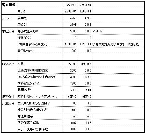
Fig.3.2.1 Analysis condition
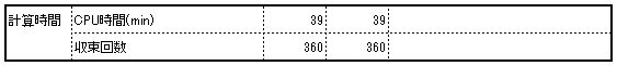
Fig.3.2.2 Calculation time and number of convergence
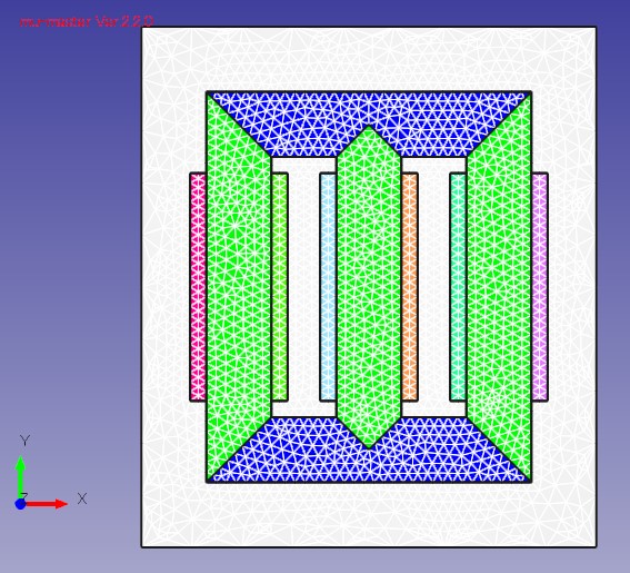
Fig.3.2.3 Mesh diagram
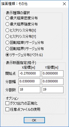
Fig.3.2.4 Evaluation points of Lissajous waveform
3. Magnetic flux line, magnetic field distribution, iron loss distribution result
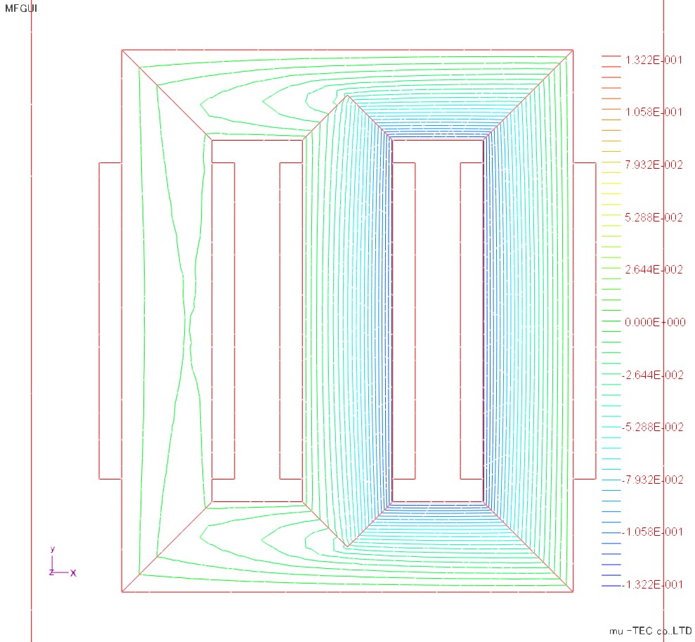
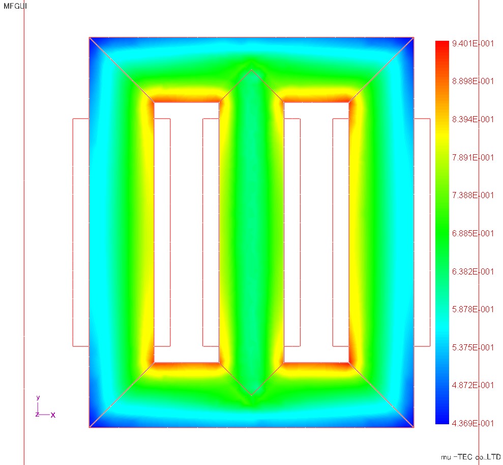
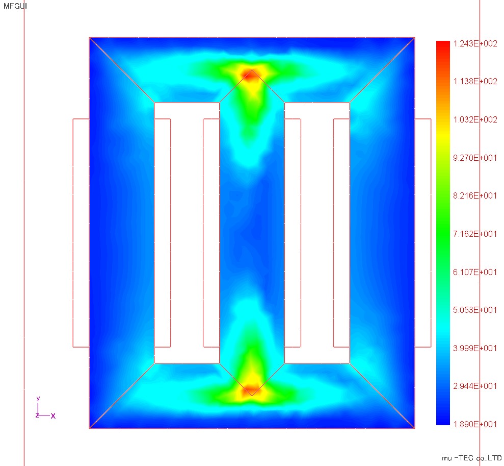
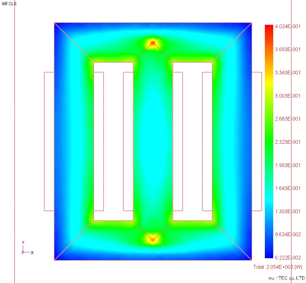
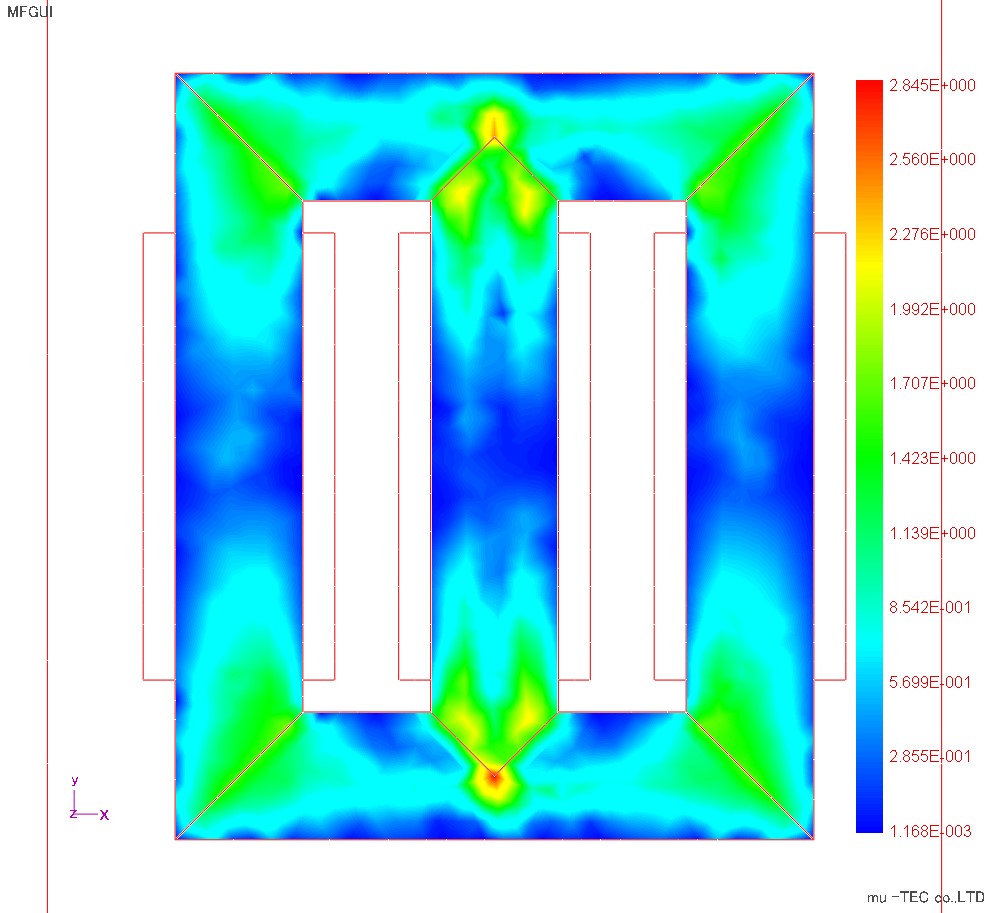
Fig.3.3.1, Fig.3.3.2, Fig.3.3.3, Fig.3.3.4 shows the magnetic flux diagram, maximum magnetic flux density distribution, maximum magnetic field strength distribution, and iron loss distribution. In the magnetic flux diagram, it can be confirmed that a magnetic flux line flows along the rolling direction of the directional material and is bent at right angles (abruptly) at the joint portion. The magnetic flux density is larger inside the window frame with a shorter magnetic path length, and 35 G 155 is larger for the steel material comparison. The maximum magnetic field intensity appears near the apex of the T-shaped joint of the upper and lower steel materials and the leg steel, and 35 G 155 is larger in the steel material comparison. In the iron loss distribution, the T type junction is large, the window frame part is large, the T type junction part is large, the influence of the magnetic field strength is large, the influence of large magnetic flux density comes out when the window frame part is large I believe that. Furthermore, in the comparison of steel materials, 35 G 155 was large, and the total iron loss was about 17% larger than 35 G 155.
 |
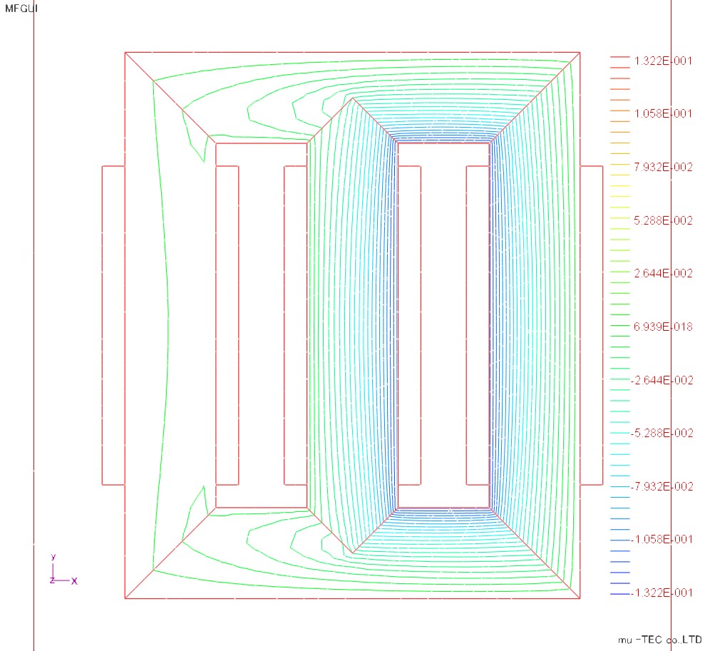 |
Fig.3.3.1 Magnetic flux diagram Left: 27P90 Right: 35G155 |
|
 |
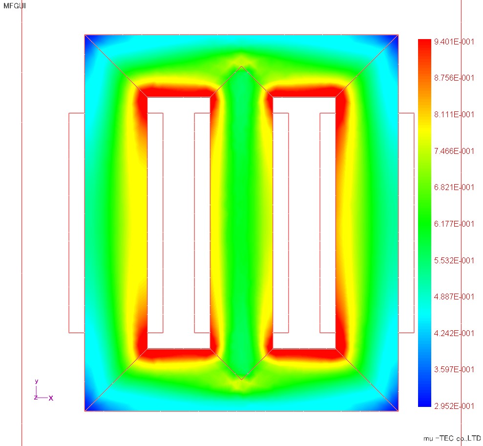 |
Fig.3.3.2 Maximum magnetic flux density distribution (indicated by maximum 0.94 T) Left: 27 P 90 Right: 35 G 155 |
|
 |
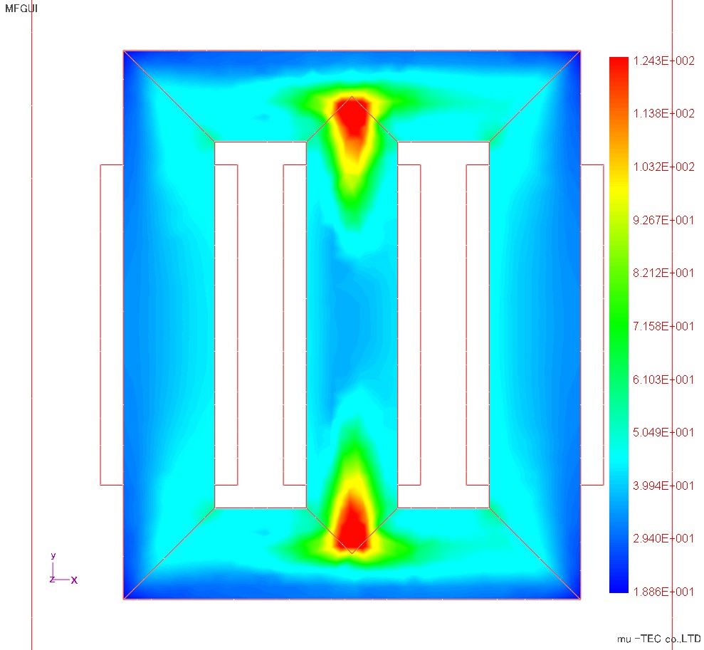 |
Fig.3.3.3 Maximum magnetic field intensity distribution (displayed at a maximum of 124 A / m) Left: 27 P 90 Right: 35 G 155 |
|
 |
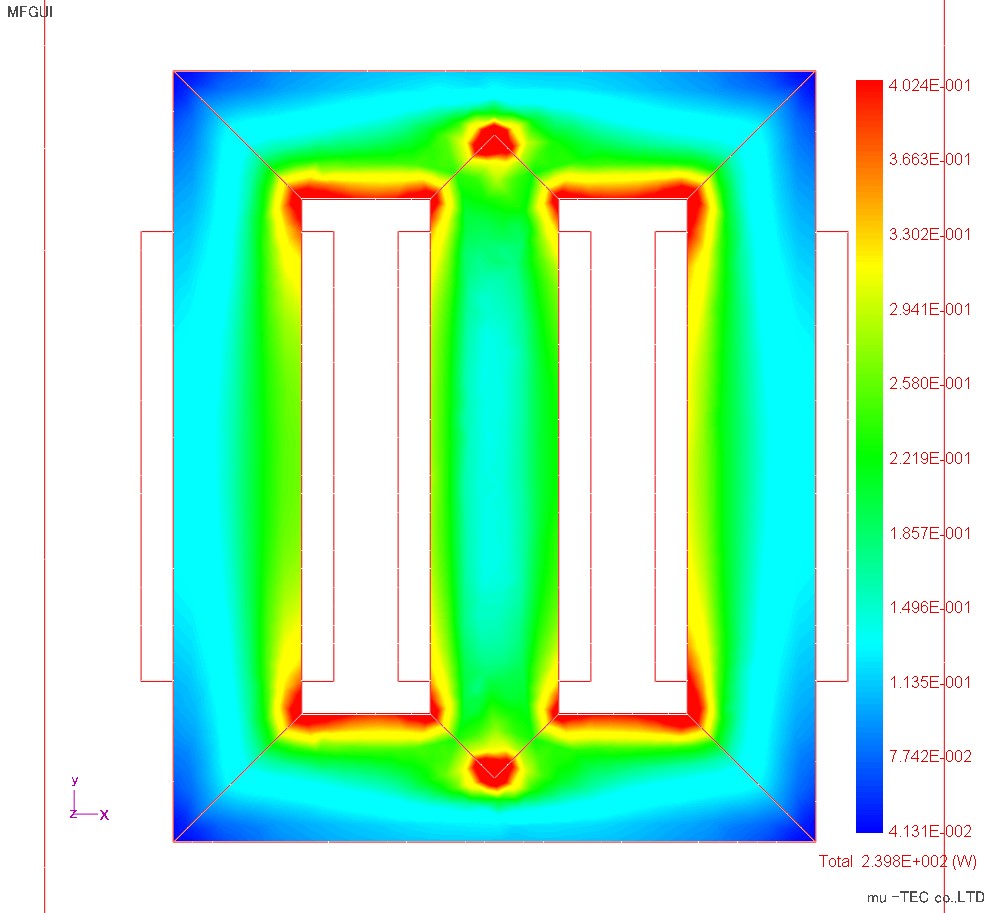 |
Fig.3.3.4 Iron loss distribution (indicated at maximum 0.4 W / kg) Total iron loss value is left: 27 P 90 205.4 (W) Right: 35 G 155 239.8 (W) |
|
4. The inclination angle θ B and the axial ratio α distribution result
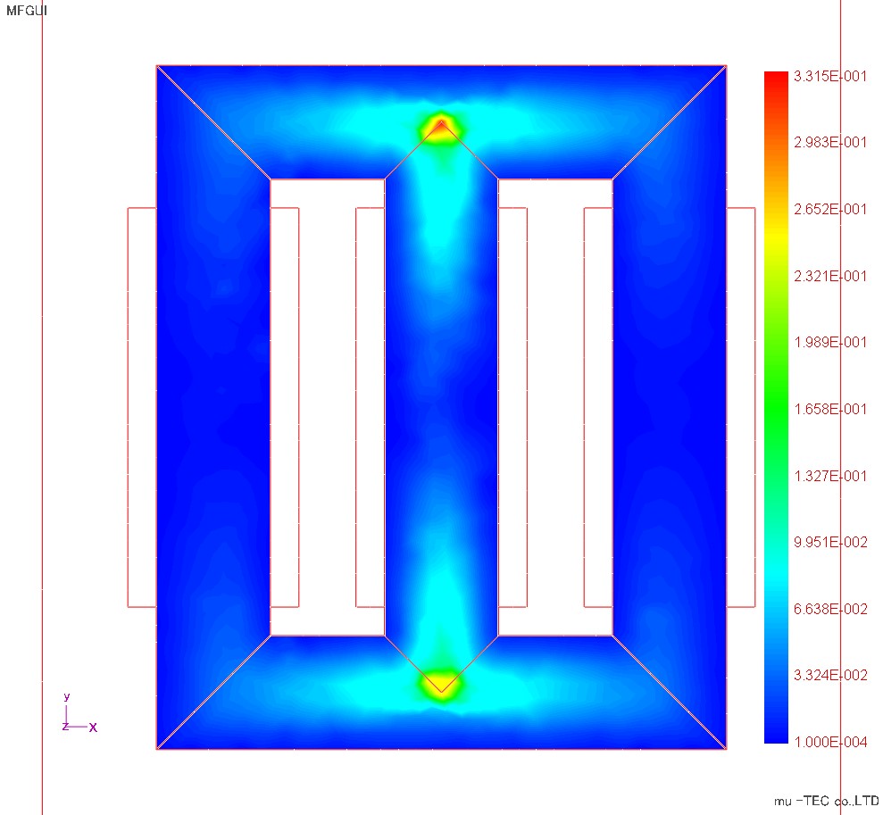
The inclination angle θb is an anticlockwise angle of the alternating magnetic flux with respect to the rolling direction, and in the case of the rotating magnetic flux, it is an angle with the direction of the maximum magnetic flux density. The inclination angle θ B distribution result is shown in Fig. The inclination angle θ B increases near the joint, because the direction of the magnetic flux density changes abruptly at the joint, it is thought that it can not completely follow the rolling direction. In the comparison of steel materials, the 35 G 155 is larger and the maximum angle is 50 °. The axial ratio α is the ratio of the major axis to the minor axis of the rotating magnetic flux, α = 1 is a perfect circle, and α = 0 is an alternating magnetic flux. The axial ratio α distribution result is shown in Fig. The maximum of the axial ratio α appears at the apex of the T-shaped joint, indicating that the rotating magnetic flux is generated here. In the comparison of steel materials, the distribution is almost the same, and the size is slightly larger for 35 G 155.
 |
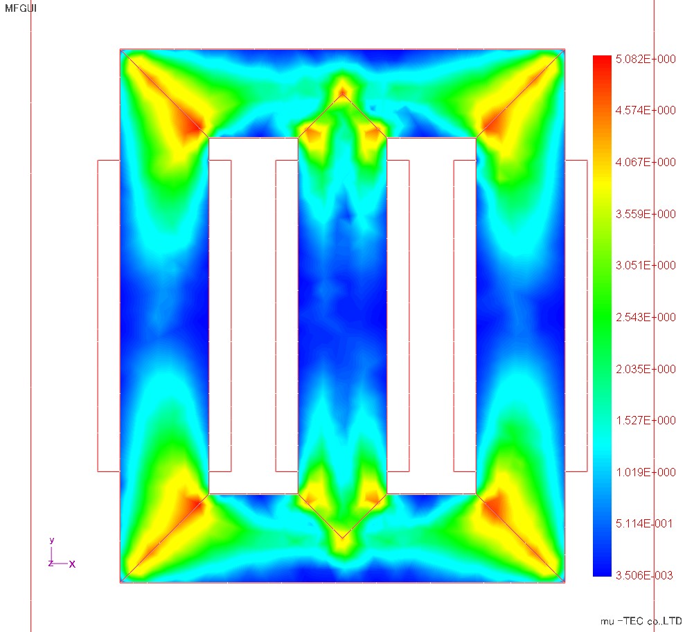 |
Fig.3.4.1 Angle of inclination θB Left: 27P 90 Maximum 28.5 degrees Right: 35 G 155 Max 50.8 degrees |
|
 |
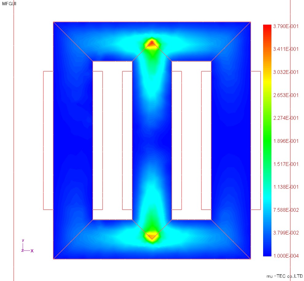 |
Fig.3.4.2 Axial ratio α Left: 27 P 90 Max. 0.33 Right: 35 G 155 Max. 0.38 |
|
5. X direction hysteresis curve result
Distribution results of the X direction hysteresis curve (with normalization, without normalization) are shown in Fig. 3.5.1 and Fig. Because X direction magnetic flux is generated in the upper steel material, the X direction hysteresis curve is increased with the upper steel material (from the diagram without normalization). An enlarged view of the blue circle in it is shown in Fig. 3.5.3, and a DB value corresponding to that part is shown in Fig. The 35 G 155 of the hysteresis curve is sleeping and the tendency of bulging tends to be seen.
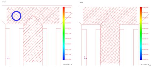
Fig.3.5.1 X direction Hiszave (normalization) Left: 27P90 right: 35G155
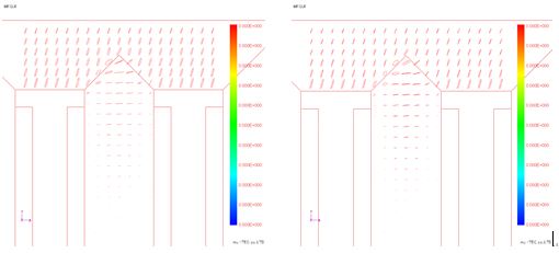
Fig.3.5.2 X direction His - curve (without normalization) Left: 27P90 Right: 35G155
 |
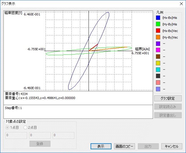 |
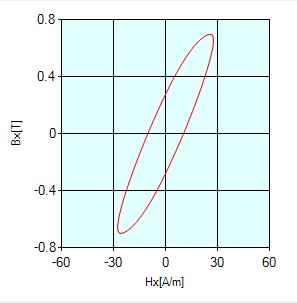
Fig.3.5.3 X direction Hiszave expansion (blue circle part) Left: 27P90 right: 35G155 |
|
 |
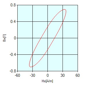 |
Fig.3.5.4 X direction Hiscarb DB value (blue circle) Left: 27P90 right: 35G155 |
|
6. Y direction hysteresis curve result
Distribution results (with normalization, no normalization) of the Y direction hysteresis curve are shown in Fig 3.6.1, Fig 3.6.2. Since Y-direction magnetic flux is generated in the leg steel, the Y-direction hysteresis curve is increased with the leg steel (from the diagram without normalization). An enlarged view of the blue circle in it is shown in Fig. The inclination of the hysteresis curve is slightly steeper in 35 G 155, and the tendency toward bulging tends to be seen.
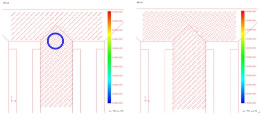
Fig.3.6.1 Y direction Hiscarb (normalization) Left: 27P90 right: 35G155
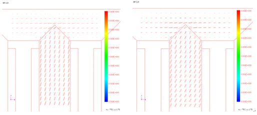
Fig.3.6.2 Y-direction His-curve (without normalization) Left: 27P90 Right: 35G155
 |
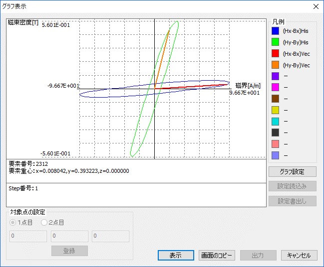 |
Fig.3.6.3 Y direction diagonal expansion (blue circle) Left: 27P90 right: 35G155 |
|
7. Lissajous waveform result
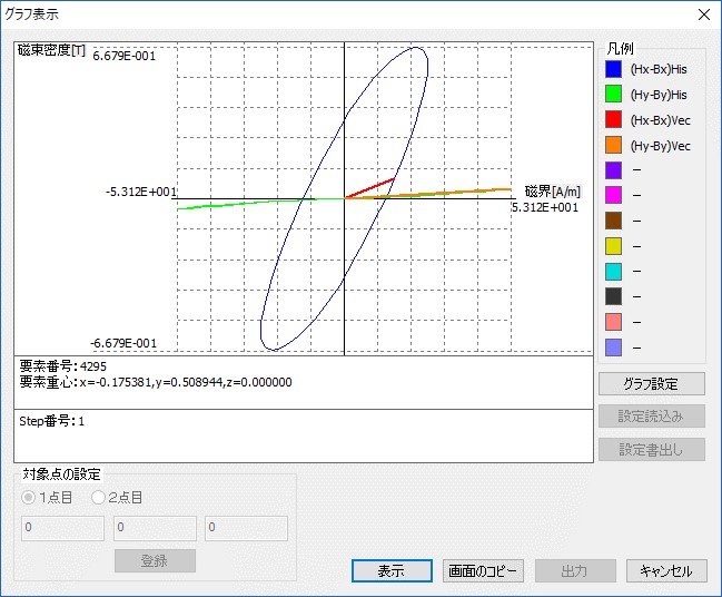
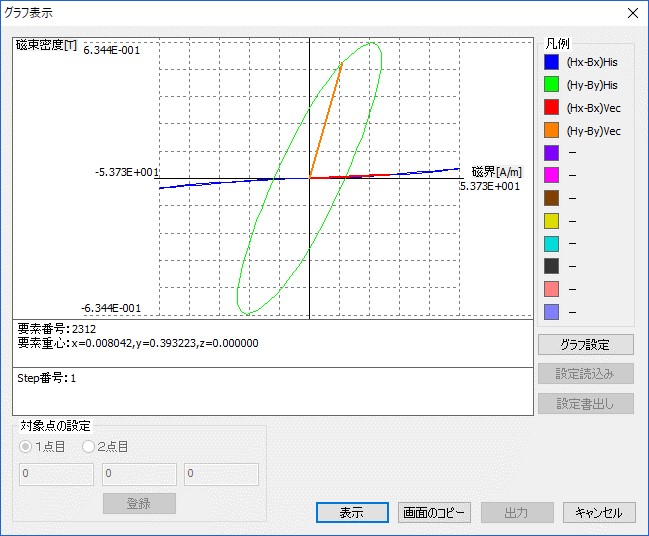
Fig.3.7.1 shows the Lissajous waveform of magnetic flux density and magnetic field strength near the T type junction. Basically, the magnetic flux density vector (red) is an alternating magnetic flux toward the rolling direction of the directional material, but it can be confirmed that the rotating magnetic flux is generated near the joint. It can be confirmed that the magnetic field strength vector (blue) shows a tendency that the magnetic flux density vector is a rotating magnetic field even in the place of the alternating magnetic flux. Next, four points (pink, blue, brown, green circle) near the apex of the T-shaped joint are confirmed in detail. An enlarged view of the pink round part is shown in Fig. Here, a large rotating magnetic flux (blue) can be confirmed at the apex of the T-shaped junction, where the magnetic field expands in the lateral direction. On the contrary, a very flat rotating magnetic field (green) is generated in the X direction of the magnetic field strength. This is because the rolling direction in this portion is the Y direction, and the magnetic resistance in the X direction is very large. An enlarged view of the blue circle is shown in Fig. This part is based on the alternating magnetic flux (blue) in the Y direction as a basis. In the steel material comparison, the tendency of the alternating magnetic flux is stronger in 27 P 90. On the other hand, the magnetic field strength (green) was a flat rotating magnetic field in the X direction, and the flatness ratio of 35 G 155 became larger. The enlarged view of the tea circle is shown in Fig. This part is where the magnetic field coming from the apex of the leg develops in the left-right direction. The magnetic flux density (blue) is a rotating magnetic flux that is flat in the X direction. The magnetic field strength (green) is a flat rotating magnetic field in the Y direction, because the rolling direction of this part is the X direction, the magnetic resistance in the Y direction is very large. The enlarged view of the green circle part is shown in Fig. In this part, the alternating magnetic flux in the X direction is the basis. The magnetic flux density (blue) is flat rotating magnetic flux in the X direction and the magnetic field strength (green) is flat rotating magnetic field in the Y direction.
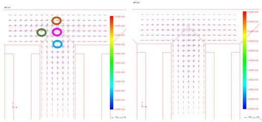
Fig.3.7.1 Lissajous waveform (red: flux density, blue: magnetic field strength) (no normalization) Left: 27P90 right: 35G155
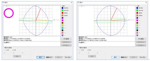
Fig.3.7.2 Pink Round Lissajous Waveform Expansion (Blue: Magnetic Flux Density, Green: Magnetic Field Strength) Left: 27 P 90 Right: 35 G 155
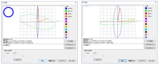
Fig.3.7.3 Blue circle Lissajous waveform expansion (blue: magnetic flux density, green: magnetic field strength) Left: 27 P 90 right: 35 G 155
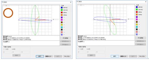
Fig.3.7.4 Brown circle part Lissajous waveform expansion (blue: magnetic flux density, green: magnetic field strength) Left: 27P90 right: 35G155
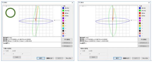
Fig.3.7.5 Green circle part Lissajous waveform expansion (blue: magnetic flux density, green: magnetic field strength) Left: 27P90 right: 35G155