


Analysis example collection (4) SPM motor (basic analysis)
table of contents
1. Analysis model and purpose
Basic analysis with the aim of iron loss distribution of SPM (surface magnet motor) is carried out. Fig. 4.1.1 and Fig. 4.1.2 show model drawings and dimension drawings. This model refers to the rotating machine of the Institute of Electrical Engineers: one of the benchmark question of investigation committee benchmark, number R 4, permanent magnet electric motor model (DC brushless motor) (technique: Chapter 486, Chapter 3). Since the rotating magnetic field is generated in the stator core, the X direction is designated as the rolling direction by the non-oriented electrical steel sheet 50 A 470, and the vector magnetic characteristic analysis is applied. Since the rotating magnetic field is not generated in the rotor, vector magnetic characteristic analysis can not be applied. This area is S45C and nonlinear analysis using a normal BH curve is performed. Voltage was input to the exciting coil and excited so that the maximum magnetic flux density became about 1.2 T.
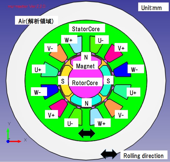
Fig.4.1.1 Transformer model
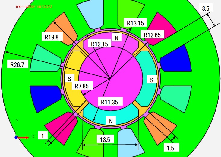
Fig.4.1.2 Dimension chart
2. Analysis conditions and calculation time
The analysis conditions are shown in Fig.4.2.1. In the mesh model, the radius of the slide is separated on the stator side and the rotor side, and the nodes are doubled. Apply periodic boundary condition to corresponding node and combine. Rotation of the rotor is achieved by shifting the pair of periodic boundary conditions in the direction of rotation. Therefore, the nodes on the slide radius are divided at an equal pitch angle. The calculation time was about 43 min (Intel Core i 5, 28 GHz machine), and the nonlinear iteration converged at 256 times (Fig. The mesh diagram is shown in Fig. 4.2.3, and the Lissajous waveform evaluation point is shown in Fig.
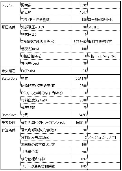
Fig.4.2.1 Analysis condition
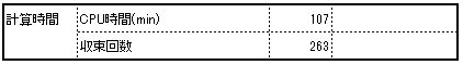
Fig.4.2.2 Calculation time and number of convergence
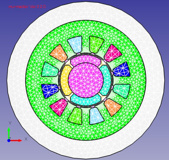
Fig.4.2.3 Mesh diagram
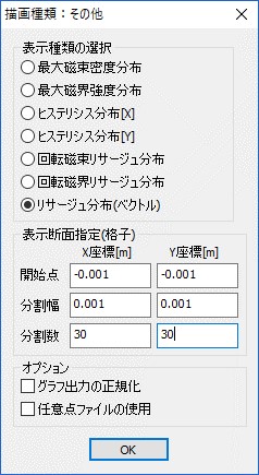
Fig.4.2.4 Evaluation points of Lissajous waveform
3. Magnetic flux line, magnetic field distribution, iron loss distribution result
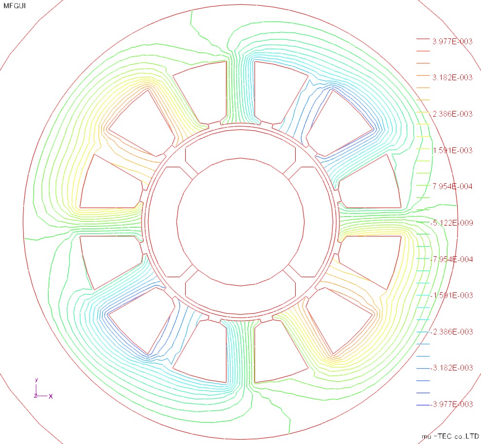
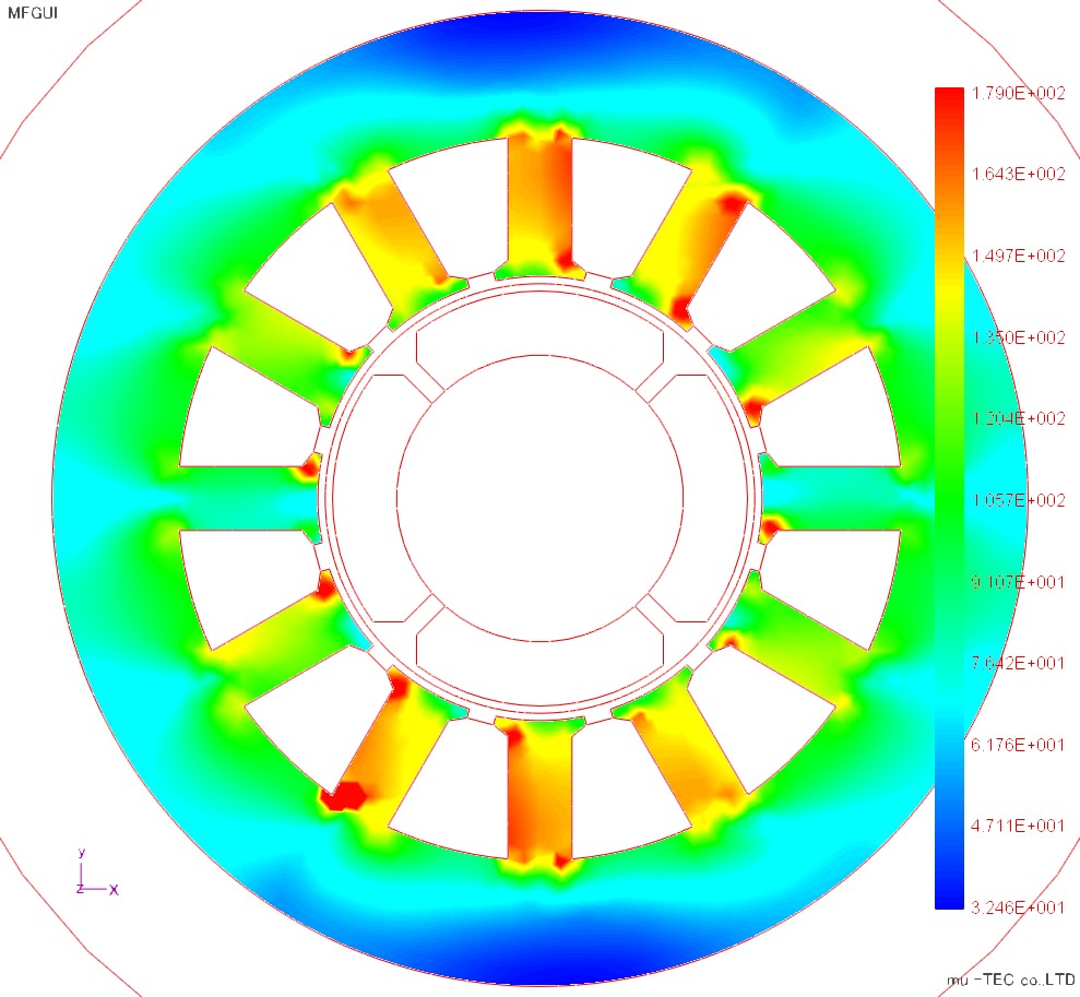
The magnetic flux diagram, the maximum magnetic flux density distribution, the maximum magnetic field strength distribution, and the iron loss distribution are shown in Fig.4.3.1 to Fig.4.3.4. Although the magnetic flux density is increased in the teeth portion and the short corner portion of the magnetic path, it is almost the same in the circumferential direction. The magnetic field strength has large teeth in the upper and lower regions, and the rolling direction is influenced by the X direction. In the iron loss distribution, the teeth portions of the upper and lower regions are increased under the influence of the magnetic field strength. In the conventional iron loss type method, since the change in the circumferential direction can not be seen similarly to the magnetic flux density distribution, the effect of vector magnetic characteristic analysis can be confirmed.
 |
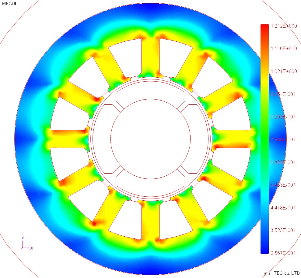 |
Fig.4.3.1 Magnetic flux diagram |
Fig.4.3.2 Maximum magnetic flux density distribution (indicated by a maximum of 1.212 T) |
 |
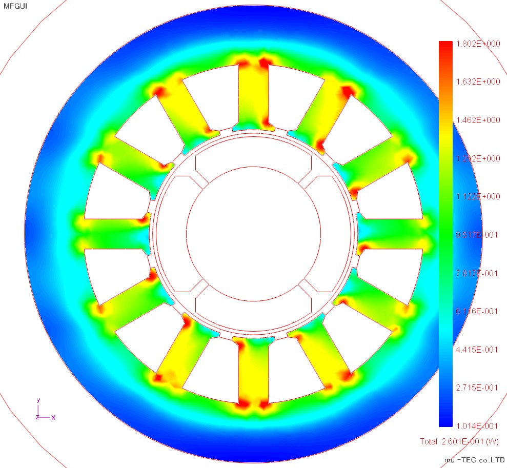 |
Fig.4.3.3 Maximum magnetic field strength distribution (indicated at maximum 179 A / m) |
Fig.4.3.4 Iron loss distribution (indicated by maximum 1.802 W / kg) Total iron loss value is 0.2601 (W) |
4. The inclination angle θ B and the axial ratio α distribution result
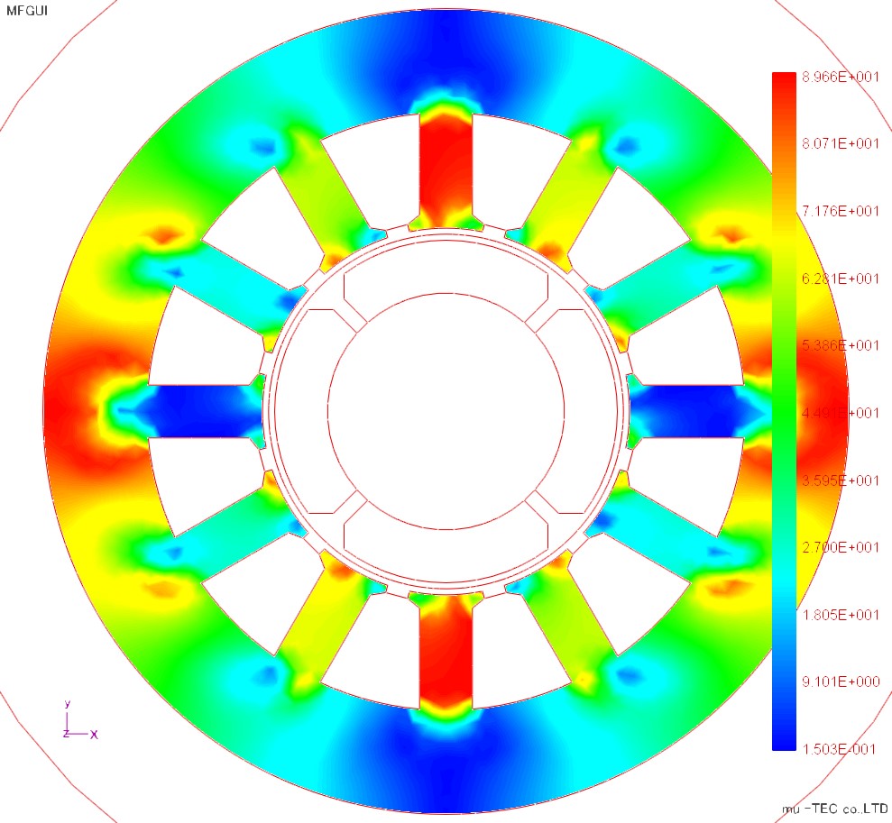
The inclination angle θb is an anticlockwise angle of the alternating magnetic flux with respect to the rolling direction, and in the case of the rotating magnetic flux, it is an angle with the direction of the maximum magnetic flux density. The inclination angle θ B distribution result is shown in Fig.4.4.1. The inclination angle θ B increases in the vicinity of the upper and lower teeth portions and the base portions of the left and right teeth portions, which can be understood from the relation between the flow of the magnetic flux and the rolling direction. The maximum angle is about 90 degrees. The axial ratio α is the ratio of the major axis to the minor axis of the rotating magnetic flux, α = 1 is a perfect circle, and α = 0 is an alternating magnetic flux. The axial ratio α distribution result is shown in Fig.4.4.2. Since the maximum of the axial ratio α is large at the base of each tooth part, especially large in the left and right regions, the rotational magnetic flux is larger in the left and right regions than in the upper and lower regions.
 |
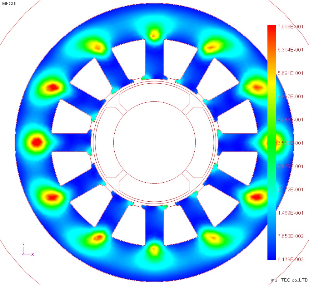 |
Fig.4.4.1 Angle of inclination θB Up to 89.6 degrees |
Fig.4.4.2 Axial ratio α Maximum 0.7 |
5. X direction hysteresis curve result
Distribution results of the X direction hysteresis curve (with normalization, without normalization) are shown in Fig. 4.5.1, Fig. Since the X direction magnetic flux is generated in the teeth part in the 3 o'clock direction, the X direction hysteresis curve is large (from the diagram without normalization).
 |
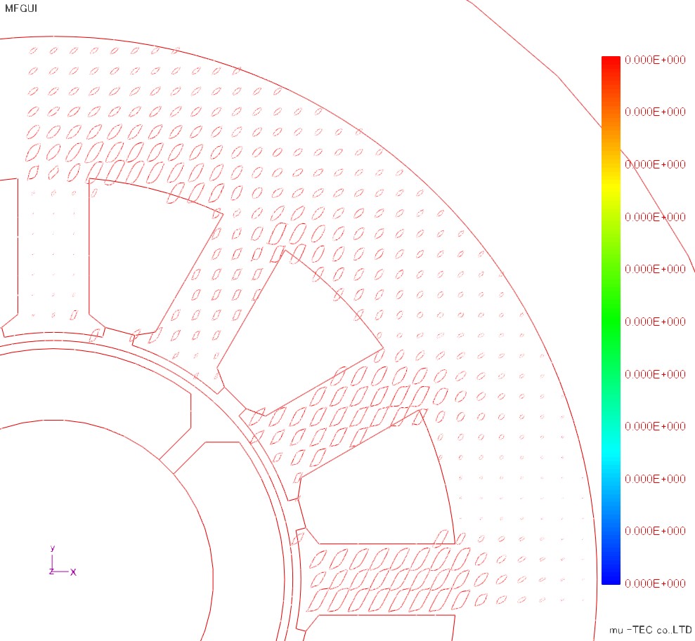 |
Fig.4.5.1 X direction Hiscarb (with normalization) |
Fig.4.5.2 X direction Hiscarb (without normalization) |
6. Y direction hysteresis curve result
Distribution results (with normalization, no normalization) of the Y direction hysteresis curve are shown in Figure 4.6.1, Fig. Y direction magnetic flux is generated in the teeth part in the 0 o'clock direction, so the Y direction hysteresis curve is large (from the diagram without normalization). An enlarged view of the teeth part is shown in Fig. In the hysteresis curve, the area on the right side of the teeth part is larger and the iron loss is larger (Fig 4.6.4). This is because the delay angle (load angle) of the magnetic pole on the rotor side with respect to the rotating magnetic field produced by the stator side is set to 30 degrees, so that the magnetic flux density passing through the right side increases.
 |
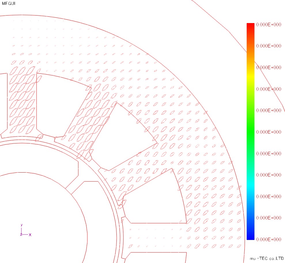 |
Fig.4.6.1 Y direction hiss curve (with normalization) |
Fig.4.6.2 Y-direction hiss curve (no normalization) |
 |
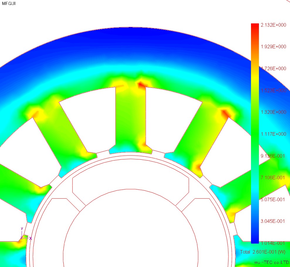 |
Fig.4.6.3 Expansion of Y direction hisection tooth part (with normalization) |
Fig.4.6.4 Iron loss distribution |
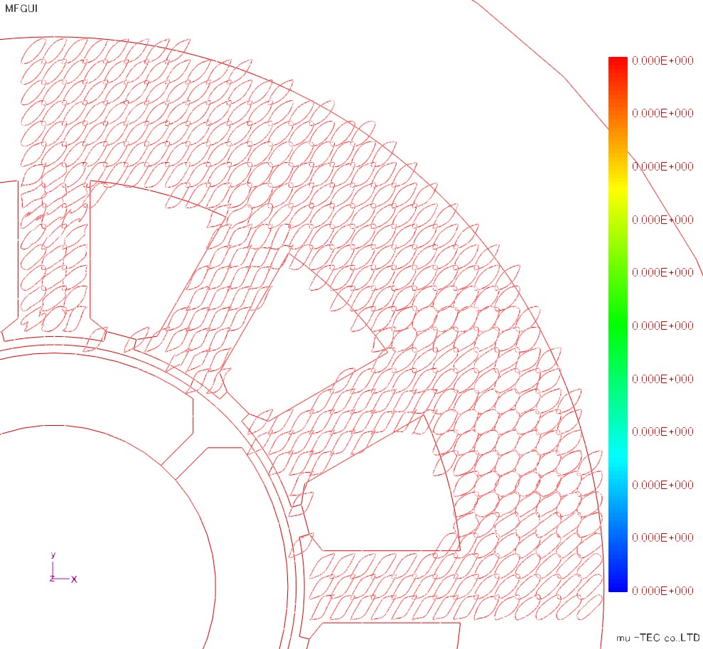
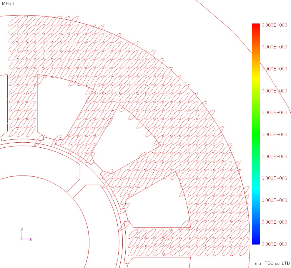
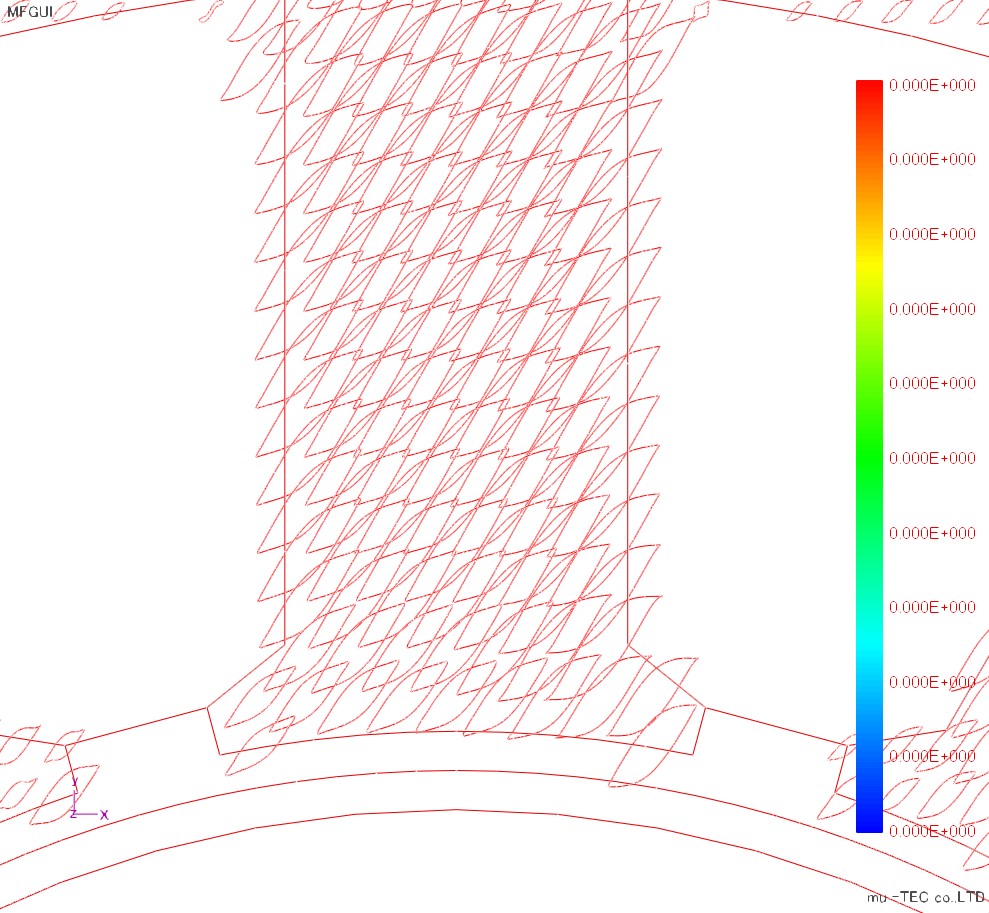
7. Lissajous waveform result
The Lissajous waveforms (with and without normalization) of magnetic flux density and magnetic field strength are shown in Fig. 4.7.1 and Fig. 4.7.2. Basically, the magnetic flux density vector (red) is an alternating magnetic flux along the flow of the magnetic flux or a rotating magnetic flux slightly bulging in the perpendicular direction, but it can be confirmed that the rotating magnetic flux is generated near the root of the tooth . It can be confirmed that the magnetic field intensity vector (blue) has a rotating magnetic field larger than the magnetic flux density vector. Next, the enlarged view of the root part of the tooth is shown in Fig. 4.7.3 to Fig. In this figure, changes in the magnetic flux density vector and the magnetic field strength vector are tracked with the change in the electrical angle. Both of them rotate in the clockwise direction, but the opening angle θBH of the magnetic flux density vector and the magnetic field intensity vector is small at the electrical angle of 0 degree of 180 degrees, and is large at 120 degrees of 300 degrees, it varies according to the electrical angle .
 |
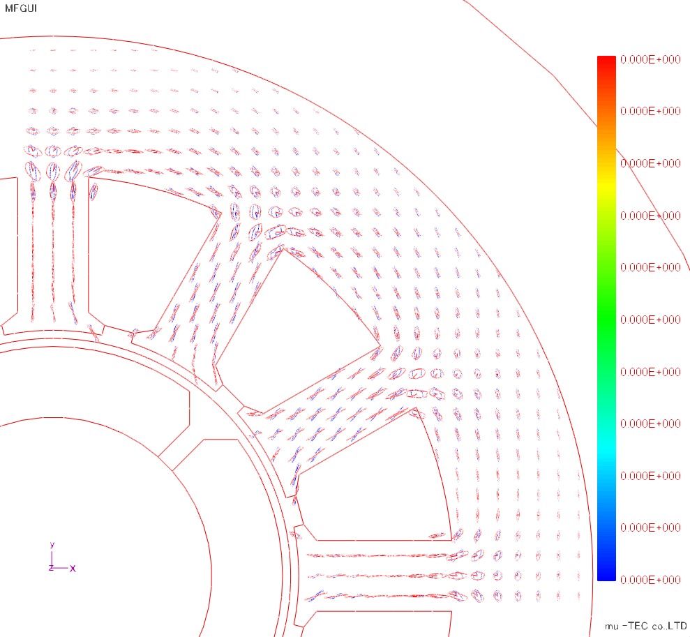 |
Fig.4.7.1 Lissajous waveform (with normalization) |
Fig.4.7.2 Lissajous waveform (no normalization) |
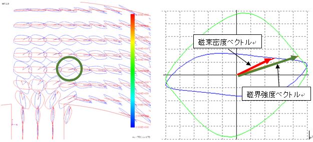
Fig.4.7.3 Lissajous vector expansion (electrical angle 0 degree)
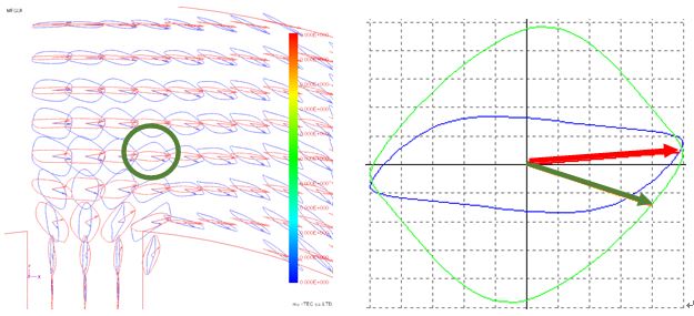
Fig.4.7.4 Lissajous vector expansion (electrical angle 60 degrees)
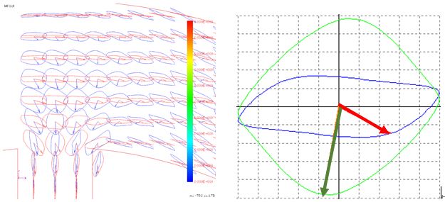
Fig.4.7.5 Lissajous vector expansion (electrical angle 120 degrees)
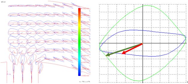
Fig.4.7.6 Lissajous vector expansion (electrical angle 180 degrees)
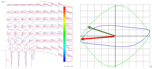
Fig.4.7.7 Lissajous vector expansion (electrical angle 240 degrees)
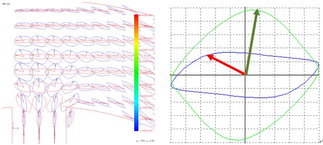
Fig.4.7.8 Lissajous vector expansion (electrical angle 300 degrees)